TABULATE [(var1|dom1) units [AND (var2|dom2) units ...]] [IF fltr]
            [FROM infile1 [AND infile2 ...]] [TO outfile1 [AND outfile2 ...]]
            [WEIGHT [OVER|PER|BY] (var4|dom4) units [AND (var5|dom5) units ...]]
            [OVER (var6|dom6) units [AND (var7|dom7) units ...]]
            [PER (var8|dom8) units [AND (var9|dom9) units ...]]
            [DISPLAY (var10|dom10) units [AND (var11|dom11) units ...]]
            [(COLLATE|ORDER*|ACCRUE) [dom12 units [val1 [val2 ...]
            [STEP units step1 [step2 ...]]]]]
PER and WEIGHT PER are new options that apply to the COPY?, COMBINE?, TOTAL?, TABULATE?, PROCESS?, and REALLOCATE commands (see Alias Table? of Streamz Language for sub-keywords under primary keywords). PER is very similar to OVER, except for when it gets applied. For output streams that are created from just a single input stream (as is always the case with the COPY, PROCESS, and REALLOCATE commands), PER and OVER give identical results. When an output stream is composed of several constituent streams, however (as can be the case with the COMBINE, TOTAL, or TABULATE commands), the effects might be different (although not necessarily). OVER is applied once for each constituent stream (you can remember this as "over and over"), whereas PER is applied just once "per" output stream. Generally, OVER will give you an average constituent rate of some sort, whereas PER will give you a combined average rate, which might be different. Detailed explanations, along with the actual formulas, are given in the associated document "Weighting.pdf". DISPLAY (alias SHOW) is another new option for the TABULATE command. It can be used to display the output values of variables other than those tabulated and collated. Variables that are simply displayed will have no effect on how the tabulations or collations are performed. They will just be output whenever they can be determined unambiguously. Specifically, an ordinary variable will be shown whenever its value is the same for all constituents of an output stream, while domain variables will be adjusted to show the encompassing domains for each output stream.
The most powerful new feature, though, is the COLLATE (alias GATHER) option and the related options ORDER (alias REORDER) and ACCRUE (alias INTEGRATE). As you can see, each one of these options has several options of its own. Some examples:
a) COLLATE
b) COLLATE time days
c) COLLATE time years 0 1 2 3 4 5 d.
d) COLLATE time months 0 1 2 3 STEP months 3*3 4*6 2*12
Explanations:
Let's assume "TABULATE WELL" is the primary command and that your input files include streams from 10 unique wells (satisfying any specified filter). Here are the results you'd get from the above options:
Now let's assume that "TABULATE WELL AND TIME (MONTHS)" is the primary command. The results of cases (b), (c), and (d) remain essentially the same, except the times will always be output by months, regardless of the units given for the collation points. Case (a) will behave quite differently, however. It will now collate all the streams that have unique combinations of WELL, starting TIME, and ending TIME. That could be any number of streams (as few as 10 or as many as the total number of input streams).
As you can see, you'll have a lot of flexibility at your disposal. As for the specific question about reporting cumulative molar productions, let's assume that you simply want monthly cumulatives for each well over a 10-year period (for example). If your input streams are already in terms of cumulatives, you would say:
TABULATE WELL, COLLATE TIME MONTH 0, STEP MONTHS 120*1
On the other hand, if your input streams are in terms of daily rates, you would simply add "WEIGHT TIME DAYS" to the above command. Then, if you decided you wanted average daily rates for each well over those monthly time periods, you would just add "OVER TIME DAYS" or (more likely) "PER TIME DAYS" to the previous command, depending on how your input data were arranged and the type of average you wanted (see Weighting.pdf for more information).
If you replace the COLLATE keyword with ORDER (leaving all other input the same), the output streams will be sorted according to the following criteria:
Highest priority: Output stream units (in case your conversions lead to differences). Amounts will come first, then Volumes, Moles, and finally Masses.
Next priorities: Tabulated variables (except those belonging to the ordered domain, if any). Priority will be assigned in the order the variables (or domains) were specified by the TABULATE command (with lower domain variables taking priority over their upper counterparts). The variables will be sorted into ascending order (numerically or alphabetically), with undefined variables coming last.
Final priority: The ordered domain, which will be sorted into ascending order.
Displayed variables will have no effect on the sorting.
The final option uses the keyword ACCRUE. If you use this in place of the ORDER keyword, each set of ordered results (having the same tabulated variables aside from the ordered domain) will be further combined into running totals before being output. All of the other previous rules for the ORDER option (as well as for the WEIGHT, OVER and PER options) still apply.
Unsure about what we mean? Need a one line definition of a term used on the website? What is a Resource? A Process?
This is the place you want to bookmark. A collection of all technical terms in the context of Pipe-It. Even Pipe-It is defined here. Use the search function to search for the term.
| TERM | EXPLANATION |
|---|---|
| Annotations | Text boxes that have no bearing on the execution of a project. They are useful in providing titles and notes to the user of the project. |
| App2Str | Format translators from 3rd party applications to Pipe-It/Streamz stream file (*.str) format. Ecl2Str (from EclipseTM) and Sen2Str (from SensorTM) are shipped with Pipe-It. Large scale usage of Pipe-It with other programs are likely to result in newer App2Str utilities. |
| Canvas | The graphical “playing field” displayed by Pipe-It. It is, by default, gray in color with an image of the Pipe-It logo in the background. There always exists the main “top level” canvas, but the user may create multiple cascading composites, each having their own canvases. |
| Characterization? | A flexible collection of components, and optionally their properties, that may be used to represent streams in stream files. Quantities of each component (of the characterization) are stored as values in stream files. Quantities may be in mass, moles, volumes, or a generic “amount”. Usually defined in simple text files that are imported into Pipe-It Streamz Library prior to use. |
| Composite | A brownish rectangle with round corners and double lines. Used to group logically related base elements (Resources, Processes or other Composites). Used to define the extent of execution of a part of a project. |
| Connectors | An elbowed (or straight) line with an arrow-head defining a connection between Resources and Processes. Connections transcending composites go via sockets but can always be tracked back to the originating Resource or Process. |
| Conversion? | A translation of streams from one characterization to another. A Streamz conversion “method” is defined in a simple file and imported into the Streamz Library, automatically connecting to pre-existing in-out characterization pairs. In case of ambiguity user assistance is needed. Once in the library, their usage is mostly automatic. |
| Linkz | The Pipe-It proprietary technology that allows the user to pin-point numbers in text (and Excel) files and denote them as variables of the Pipe-It project. An intuitive and robust fingerprinting method is used customized by the user to uniquely define the location of the number with respect to surrounding “tokens”. These numbers can then be read and written by Pipe-It. Repeatedly and without regard to their original line in the file. Columns/Rows and whole matrices are supported. Text tokens too. |
| MapLinkz | The customized Pipe-It process that manages mapping of Linkz variables from one resource to another (read one file to another). Enables quick and easy way to pass results of one application as input to another. |
| Optimizer | Pipe-It “supervisor” that can control multiple launches of the underlying Pipe-It model. Works with Linkz variables to cause values to written (VAR and AUX) to files before the launch of the model, or cause the values to be read (AUX, OBJ and KPI) after the completion of the model run. Can launch multiple user-specified (Case Matrix) or automated (Solver Driven) executions of the underlying model. The underlying model may be the full project or parts of it (Composites). |
| Petrostreamz | Is the Trondheim, Norway based company that develops and sells Pipe-It. It also offers consultancy and training related to Pipe-It. |
| Pipe-It | Is the software application developed and sold by Petrostreamz AS. Conceptually it allows piping together the various computational models used in a value chain, or workflow, into an integrated & automated project. Once integrated and automated, it allows the user to optimize on any key result computed by the integrated poject. |
| Pipe-It model | Strictly the model part of a Pipe-It project. The Pipe-It Project Model (ppm) file is the main entry point for Pipe-It’s Runner and is only needed to execute a project. For typical usage of Pipe-It, the term model is interchangeably used with the term project. |
| Pipe-It project | A collection of files that represent all the graphical (*.ppv) and logical (*.ppm) parts of a Pipe-It data-set. The Pipe-It Project View (ppv) file is the main entry point into Pipe-It and is the point of interaction for the user. Ppv files are associated with Pipe-It upon installation and double-clicking a project’s ppv file loads it into Pipe-It. |
| Pipe-Itc | The command line version of Pipe-It, enabling Pipe-It to be called from any 3rd party application that can launch applications. Since Pipe-It is such an application, Pipe-It can call Pipe-It itself! |
| Plotz | The visualization tool of Pipe-It. Runs as any 3rd party application. Can make 2-d plots of any tabulated data in text or Excel files. Can easily mix-n-match. Special handling of stream files allows users to be up-and-running with most frequent of Resources. Command line usage allows dump of scores created plots as PDF (or image) files ready for reports or presentations. |
| Process | A greenish oval. Represents a launch of an application (program, script etc.) from within Pipe-It. Can only connect to Resources on input/output, never directly to another Process. |
| Resource | A pale-bluish rectangle with round corners. Can be dropped from the toolbar using an icon of the same appearance. Represents a file on the disk. If no file is specified, it will report a broken status to the Runner. |
| Runner | Often called the “brain” of Pipe-It, it is the hidden entity that come into play when the user hits the Run (or Play) button on the Pipe-It toolbar. It analyses the myriad of interconnected Pipe-It Resources, Processes and Composites and determines the most efficient way of launching the entire project. All dependencies are worked out and possibilities of parallel/sequential executions considered. It sets up the queue of resources & applications to be “run”, causing the dependent applications to be waiting for the completion of upstream portions of the project. |
| Sockets | Connection ports that drive the connectors in and out of composites. Also the connections points on Resources and Processes. Single Input and Output sockets pre-exists on each such graphical element, more of each type can be added and renamed by the user. |
| Solver | A Pipe-It supplied or user plugged-in algorithm to control the multiple launches of Pipe-It from the Optimizer automatically driving the currently selected OBJ (Objective) to a maximum, minimum or first-feasible value. User specified bounds of all variables (VAR/AUX/KPI) will be honored during the optimization. |
| Stream files | Tab-delimited text files following rules of Streamz. Contain a header section followed by stream data that can easily run into millions of streams. Each line is a single stream. Each stream contains optional “tags” of variables followed by quantity of all components making up the stream. |
| Streamz | Is the petroleum engineering application package with Pipe-It that excels in performing efficient and consistent petroleum streams management. It is often referred to as “engine” of Pipe-It. |
| Streamz Copier | Copies of all streams from all incoming stream files to all connected output stream files unless filters are invoked. Automatically performs characterization conversions if needed. |
| Streamz Generic | A user specified Stream management “task” implemented as a ready-to-run Pipe-It Process. All connected stream file Resources, and their corresponding characterizations, are made available on-the-fly. The user can concentrate on writing Streamz “code” to define the non-vanilla task at hand. Great for learning and validating Streamz commands. |
| Streamz Processes | These are a collection of automated ready-to-run Streamz tasks embedded into Pipe-It to get the user up-and-running with streams management. |
| Streamz Tabulator | Aggregates incoming streams, whether from a single or multiple stream file to the produced, usually smaller, aggregated stream files. Conversions are performed automatically. Typical usage: aggregate well streams to field streams. |
| Strexzel | Stream file editor allowing manipulation of existing Streamz variables and/or components, including mathematical manipulations. All such actions are recorded in Macros that can be used on command-line mode in Pipe-It with no user interference. Sum of Squares of differences (SSQ) between columns of stream data can easily be computed allowing, for example, history matching of measured data by optimizing the computational model. |
Links disappeared in the Optimizer
Linkz file format changed starting with Pipe-It 1.0. Pipe-It 1.0 can read the old format and writes only to new format (link@file). This format is used in all later versions. This version (1.0) should be used for transition of projects created before 2011 and make them compatible with the current version.
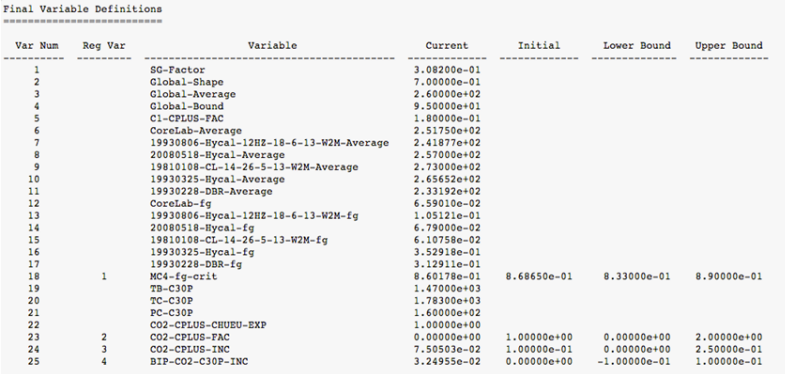
Output of PhazeComp application looks in such way:
Problem of locating values of variables which are based in fourth column "Current" is related to possibility of presence of numbers in "Reg Var" column. Then with appearing a number in the column, the position of token can be shifted and you get wrong value of your variable.
We need to avoid of considering numbers in "Reg Var" as tokens. For this you need to change delimiters regular expression. Because value of variable is definitely larger than 2 digits, we can just ignore all tokens with length less than 3 symbols. For this, in delimiters dialog, change TOKEN REGEXP
[^$delimiters]+ to [^$delimiters]{3,}
It means that instead of "+" (which means at least one symbol and more) linkz will look for "{3,}" (which means at least three symbols and more).
Then first two columns will be ignored and tokens are counted from "Variable" column.
Pipe-It is built to launch any 3rd party application like Eclipse1, Hysys2, VIP3, OLGA4 and others via the Program (Script). If the program expects command line argument (e.g. file names) and/or options (switches), they can be supplied. If the program binary (executable) is not on the system path then the entire path to the executable should be included. Quotes should be used if spaces are part of the path.
Example with Eclipse, assuming eclrun is on the path:
eclrun Eclipse "ODEHIMPES_PSM"
Example with Olga, where the executable is not on the path:
"c:\Program Files (x86)\SPT Group\OLGA 7.2.2\opi.exe" "Hydrate.genkey"
Pipe-It can use resource references to make the command line flexible and reusable.
If a 3rd party application is used frequently then Pipe-It’s Script Assistant can be used to create a short-cut on the toolbar and the application appears tightly embedded into Pipe-It. It’s usage becomes as simple as drag and drop.
Modifying data used by these applications and using results produced by these applications is as simple as using Linkz on the application’s input and output files.
Launching application that do not have text files for interaction is accomplished by wrapping the launch in a COM-complaint scripting language. Windows ships with the Windows Scripting Host (WHS) that can read and execute *.vbs files to accomplish this. If the user has other scripting environments installed on the computer where Pipe-It is to be used, for example Ruby, Perl, Python etc., any & all such systems can be used instead.
1Eclipse is trademark of Schlumberger Ltd.
2Hysys is treademark of AspenTech Inc.
3VIP is trade mark Landmark Graphics Corp.
4OLGA is the trademark of Scandpower Technology AS.
The Pipe-It created resource files (*.str files) are tab delimited and can readily be opened in a spreadsheet program like Microsoft Excel. The Pipe-It scripter command can be set to execute at following command, where one or more .str files can be specified before the .xls file that will use the data from these files:
"C:/Program Files (x86)/Microsoft Office/Office14/EXCEL.EXE" "OUTPUT-STR\ VLC2.str" "PolyFit.xls"
A simpler way, if you do not want to find out the location of Excel, would be:
Cmd /c Start Excel "OUTPUT-STR\ VLC2.str" "PolyFit.xls"
This causes Excel to behave as it is part of Pipe-It since the execution continues as soon as the instance of Excel is closed.
Pipe-It provides the user with a set of tools to manage the conversion of information among a multitude of models handling fluid streams. This software is developed to be very flexible to use. It can perform automated, multi-step conversions using batch scripts on a large number of streams. The package consists of a GUI for visually piping together a project, running external models to generate or import fluid streams, powered by the core program Streamz. This manual will get the user up and running with the Streamz program using a typical data set and explains the use of each command as they are encountered.
Any reference to "Streamz" in the text refers to the Streamz program. To distinguish between different kinds of text, we use a few typographical conventions:
Upper case, bold font is used for Streamz keywords mentioned in the text:
CONVERT, TITLE, MOLES, COPY
User-specified data to Streamz keywords are in italics:
TITLE title_string
Portions of an actual data-set used in this document are in Courier font, and enclosed within a box:
title 'Example conversion of Black-Oil streams'
subtitle 'Converted to 6 component EOS'
Keyword types:
Command – primary keyword that introduces instructions.
Sub-command – sub-level keyword that introduces further instructions.
Option – sub-level keyword that sets parameters.
Arguments – user-specified input to a keyword.
Streamz is a generic program to convert fluid streams from one characterization to another. A fluid stream is any collection of data containing information about the amounts of the constituents of a petroleum fluid, and any other associated information like origin, pressure, temperature, etc. A characterization is a definition of the names of components making up the fluid stream and, in most cases, their molecular weights. Exceptions include black-oil streams, which do not have associated molecular weights. Equation-of-state (EOS) characterizations may also include critical properties and binary interaction parameters.
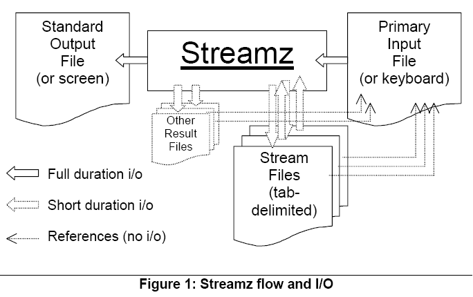
The user controls a run of Streamz via one or more nested driver files, the first of which is the Primary Input file. This file (through possible inclusion of other driver files) names the fluid characterizations, describes their properties, and defines conversions between them. It allows the user to specify the opening of stream files containing the streams for particular characterizations, and also allows instructions for filtering, combining and copying streams from one file to another. This interaction of Streamz with various files is depicted in Figure 1. Instructions are in the form of commands, sub-commands, options and arguments. All keywords and arguments are case insensitive for recognition purposes, but retain their user-specified cases otherwise (in particular for arguments such as title strings and file names). The program automatically invokes conversions among the required characterizations. Typically, various pre-processors generate the program commands, thereby ensuring that the syntax is correct.
Streamz can be invoked by using the Streamz utility in Pipe-It, or from the operating system's command line using the program name Streamz. Up to two command-line arguments can follow the Streamz command. The first argument is the name of the Primary Input file, which contains the instructions and keywords to the Streamz program. The second argument is the name of the Standard Output file, to which the program will write various messages about its execution. Path information included with the file names will be considered relative to the current working directory from which the Streamz command was issued. Streamz normally requires additional input from one or more stream files and can generate other "result" files, but these can only be specified from within the Primary Input file.
Streamz InputFile OutputFile
Invoking the program with only the first argument results in a prompt to the user (in the form of a simple text prompt or a standard file dialog box, depending on the operating system) to supply the name of the Standard Output file. If the prompt is canceled, there will be no Standard Output file. If "@" (without the quotes) is given in response to the file dialog box, the Standard Output will be redirected to the screen. Invoking the program with no arguments results in prompts for both the Primary Input and Standard Output files, in that order.
This section steps through the "hows" and "whys" of a typical Primary Input file to Streamz. This input file is an example of a typical usage of the Streamz program, and contains some of the most used keywords and their options. This data set is designed to give the first time user a template to start creating his/her own input files that allow using the program straight away. This section will list the full data set and then step through it line-by-line (or portion-by-portion), explaining the syntax and usage of each keyword and option.
The data set is set up to first convert streams, in the form of surface oil and gas volumes, from a popular black-oil reservoir simulator (Eclipse 100) into 6-component molar-rate streams. Next, a conversion to 6-component mass-rate streams is performed. The 6-component molar-rate streams are then converted to 17-component molar-rate streams required by a process simulator.
Title 'A data-set for a rich gas condensate field, Opitz'
TITLE 'Black-oil to EOS-6 Conversion'

CHAR 'Opitz BO'
NAME
SO
SG

STREAMFILE INP1:  INPUT "OpitzBO.str"
CHAR 'Opitz EOS-6'
NAME           MW
X1               18.640
X2               58.890
X3              112.420
CN1             179.980
CN2             310.000
CN3             480.000

CONVERT 'Opitz BO' from VOLUMES to MOLES
SET	PRES	(bar)	422.073
SPLIT	SO	X1	 3.62E-03	 8.28E-01	 1.01E+00
				 9.36E-01	 1.28E+00	 2.15E-01
SPLIT	SG	X1	 3.84E-02	 4.52E-03	 1.06E-03
				 2.37E-04	-5.15E-04	-2.35E-04
SET	PRES	(bar)	400
SPLIT	SO	X1	-1.44E-02	 8.74E-01	 1.06E+00
				 9.68E-01	 1.28E+00	 1.76E-01
SPLIT	SG	X1	 3.84E-02	 4.45E-03	 9.89E-04
				 1.89E-04	-5.24E-04	-1.75E-04
SET	PRES	(bar)	300
SPLIT	SO	X1	-9.77E-02	 1.03E+00	 1.24E+00
				 1.07E+00	 1.22E+00	 9.83E-02
SPLIT	SG	X1	 3.85E-02	 4.21E-03	 7.10E-04
				 3.84E-05	-4.13E-04	-5.18E-05
SET	PRES	(bar)	200
SPLIT	SO	X1	-1.77E-01	 1.13E+00	 1.42E+00
				 1.14E+00	 1.12E+00	 7.78E-02
SPLIT	SG	X1	 3.84E-02	 4.05E-03	 4.52E-04
				-3.97E-05	-2.32E-04	-1.89E-05
SET	PRES	(bar)	100
SPLIT	SO	X1	-1.98E-01	 1.09E+00	 1.58E+00
				 1.16E+00	 1.05E+00	 7.17E-02
SPLIT	SG	X1	 3.82E-02	 4.12E-03	 2.57E-04
				-5.58E-05	-1.10E-04	-7.73E-06
SET	PRES	(bar)	50
SPLIT	SO	X1	-1.27E-01	 8.11E-01	 1.62E+00
				 1.20E+00	 1.07E+00	 7.26E-02
SPLIT	SG	X1	 3.79E-02	 4.52E-03	 2.37E-04
				-6.83E-05	-1.00E-04	-6.87E-06


STREAMFILE OUT1:  OUTPUT 'OpitzEOS6z.str'

COPY

STREAMFILE INP1:  CLOSE
STREAMFILE OUT1:  CLOSE

TITLE 'Opitz EOS-6 to EOS-17 Conversion'
TITLE '(kg-moles/day of EOS-6 to kg-moles/hr of EOS-17)'
TITLE '(also to kg/hr of EOS-6)'

STREAMFILE  INP1: INPUT  'OpitzEOS6z.str'
STREAMFILE  OUT1: OUTPUT 'OpitzEOS6w.str'

CONVERT 'Opitz EOS-6' to MASS

CHAR 'Opitz EOS-17'
NAME     MW     FULLNAME
CO2             'CARBON DIOXIDE'
N2              'NITROGEN      '
C1              'METHANE       '
C2              'ETHANE        '
C3              'PROPANE       '
IC4             'ISOBUTANE     '
C4              'N-BUTANE      '
IC5             '2-METHYL BUTANE'
C5              'N-PENTANE      '
C6     84.198   'HEXANES        '
C7     97.464
C8     111.251
C9     125.799
C10    139.157
CN1    180.000
CN2    310.000
CN3    480.000

CONVERT 'Opitz EOS-6' from MOLES to MOLES, conserve MASS

GAMMA X3 C7, FILE GAM1
SHAPE 1.570, AVERAGE 1.0, BOUND 0.662693471, ORIGIN 1.0

SET PRES 423 bar
SPLIT X1 CO2   0.03514 0.00462 0.84342 0.11682
SPLIT X2 C3    0.50204 0.07055 0.19427 0.05624 0.08078 0.09611

SET PRES 373.3 bar
SPLIT X1 CO2   0.03459 0.00485 0.84757 0.11299
SPLIT X2 C3    0.51820 0.07066 0.19165 0.05460 0.07709 0.08779

SET PRES 318.2 bar
SPLIT X1 CO2   0.03397 0.00492 0.85170 0.10941
SPLIT X2 C3    0.53182 0.07159 0.19091 0.05227 0.07273 0.08068

SET PRES 263 bar
SPLIT X1 CO2   0.03396 0.00492 0.85388 0.10725
SPLIT X2 C3    0.54201 0.07101 0.18935 0.05089 0.07101 0.07574

SET PRES 207.8 bar
SPLIT X1 CO2   0.03378 0.00495 0.85473 0.10653
SPLIT X2 C3    0.54935 0.07134 0.19025 0.04875 0.06897 0.07134

SET PRES 152.7 bar
SPLIT X1 CO2   0.03429 0.00480 0.85325 0.10766
SPLIT X2 C3    0.55334 0.07151 0.19109 0.04924 0.06800 0.06682

SET PRES 97.5 bar
SPLIT X1 CO2   0.03509 0.00469 0.84823 0.11198
SPLIT X2 C3    0.55519 0.07285 0.18874 0.05077 0.06843 0.06402

SET PRES 49.3 bar
SPLIT X1 CO2   0.03604 0.00432 0.83710 0.12254
SPLIT X2 C3    0.55296 0.07289 0.19728 0.04956 0.06706 0.06025

STREAMFILE OUT2:  OUTPUT 'OpitzEOS17z.str'

GAMMAFILE  GAM1:  OPEN 'OpitzEOS6.gam'
NEWSFILE  NWS1:  OPEN 'OpitzEOS17.nws', USER AAZ

COPY, SCALING 0.041666667 ;(convert daily to hourly production)
This section steps through the Primary Input file presented in the previous section.
Title 'A data-set for a rich gas condensate field, Opitz'
TITLE 'Black-oil to EOS-6 Conversion'
The purpose of the TITLE command is to print a boxed title to the standard output file. The quoted string following the TITLE keyword is centered within a box made up of asterisk (*) characters. The box expands to accommodate the full length of the string. This may be used to visually separate different tasks being run from the same input file. A sub-command recognized within the context of TITLE is SUBTITLE (also given by a subsequent TITLE keyword, as illustrated above). Each of these sub-commands prints its line of text within the same box as the primary TITLE text. Using SUBTITLE after another keyword has been used (i.e., outside the context of the TITLE command) will result in an error.
CHAR 'Opitz BO'
NAME
SO
SG
The CHAR command names a fluid characterization. In the present example, the characterization_name "Opitz BO" is defined.
The NAME sub-keyword triggers the tabular input of an EOS property table, which defines the names and properties (such as molecular weights and critical parameters) of the components that make up the characterization. Because a black-oil characterization is being defined in this example, the property table consists of only the component names. In this case, the names given to the two components are "SO" and "SG" (Surface Oil and Surface Gas). A detailed discussion of the property table is included later.
STREAMFILE INP1: INPUT "OpitzBO.str"
The STREAMFILE keyword initiates the opening of a stream file for either input or output. The first argument to the keyword is a file_nickname (INP1 used here). The sub-command INPUT directs that an existing file is to be opened for input. Its argument is either the actual file name ("OpitzBO.str" in our example case) or else the keyword PROMPT, in case the user wants to be prompted interactively for the actual file name. If the file name is entered here, and contains blanks or unusual punctuation, it should be quoted. It may contain OS specific path directives if the file is in another directory, relative to the current input file. The information in the file being opened should correspond to the "current" characterization. The current characterization is the one just defined (or made "current" with the RESTORE command, followed by the appropriate char_name). In our case it is the "Opitz BO" characterization with two components. The stream data in the file being opened with this STREAMFILE command should contain the quantity information for two components only.
CHAR 'Opitz EOS-6'
NAME           MW
X1               18.640
X2               58.890
X3              112.420
CN1             179.980
CN2             310.000
CN3             480.000
Here we have the definition of a second characterization using the CHAR command. We need two defined characterizations to convert from one to the other. This is an EOS characterization named "Opitz EOS-6" with 6 components. The NAME sub-keyword triggers tabular input of an EOS property table and defines the properties of the components that make up this characterization. This tabular input scheme is very flexible, allowing any of the component properties (including their NAME) to be input in any order. Each property is identified by a heading keyword. For example, MW indicates molecular weight. The only constraint of the tabular input scheme is that any entries in the table that belong to a particular heading (i.e., property) should line up with the heading. This allows unknown entries to be left blank without misaligning the rest of the table. The specific rules for lining up the table are described in Appendix A of the Streamz Reference Manual. The name of each component is listed under the NAME heading. The value of any other property corresponding to that component is entered in the same row, lined up under the heading corresponding to the desired property. In our example case, the molecular weight of X3 is 112.420. This input scheme is designed to enable cut-and-paste from any other data file or spreadsheet with minimal editing. The example requires only the NAME and MW properties but input of a full EOS property table is also allowed for forward compatibility.
CONVERT 'Opitz BO' from VOLUMES to MOLES
The CONVERT keyword initiates the definition of a conversion procedure to convert streams corresponding to an input characterization into streams corresponding to an output characterization. The first argument to the keyword is the name of the input characterization (in this case "Opitz BO"). This must have been previously defined. The output characterization is the "current" characterization (the one defined last or made "current" by the RESTORE command). The FROM option defines the input units expected by the conversion procedure. Conversion will be possible only for input streams specified in these (or compatible) units. Four units are currently understood, namely MASS, MOLES, VOLUMES, and AMOUNT. The FROM units should match those in the corresponding input stream files (MASS and MOLES are compatible if the component molecular weights have been defined). The actual streams may be in more specific, dimensional units, which may also denote rates, concentrations, fluxes, etc. For example, kgmol, lbmol/day, gmole/cc, or lbmol/ft2/sec would all fall under the category of MOLES. The true, dimensional units are not relevant to the program, but should be kept track of by the user, so as not to confuse lbmol/day with kgmol/hr, for example. We use VOLUMES here because we know that the input streams are in Sm3/D (i.e. volumetric rates). The TO option specifies the units of the output streams. A CONSERVE option to the CONVERT command will be discussed later in this section. If the FROM units are not specified, they will default to the TO units, the CONSERVE units, or MOLES, in that order of preference. Then, if the TO or CONSERVE units have not been specified, they will default to the FROM units.
SET	PRES	(bar)	422.073
SPLIT	SO	X1	 3.62E-03	 8.28E-01	 1.01E+00
				 9.36E-01	 1.28E+00	 2.15E-01
SPLIT	SG	X1	 3.84E-02	 4.52E-03	 1.06E-03
				 2.37E-04	-5.15E-04	-2.35E-04
.
.
.

SET	PRES	(bar)	50
SPLIT	SO	X1	-1.27E-01	 8.11E-01	 1.62E+00
				 1.20E+00	 1.07E+00	 7.26E-02
SPLIT	SG	X1	 3.79E-02	 4.52E-03	 2.37E-04
				-6.83E-05	-1.00E-04	-6.87E-06
One way to convert an input stream to an output stream is through a set of split factors. Each split factor specifies the portion of a given input component that partitions into a given output component. Each component (input or output) may have several split factors associated with it and the split factors may be functions of one or more control variables. Streamz handles the input of these split factors by means of the SET and SPLIT (or DELUMP) keywords, which are discussed in this section. Examples are shown in the above extract, which contains only a portion of the relevant part of the data-set (missing portions are replaced by dots).
The SET sub-command is known within the context of the CONVERT command and is used to specify control variables and set their values. Here we designate the previously defined pressure variable "PRES" (defined in our input stream file by the VARIABLE command) as our one control variable and set its value initially to 422.073 bar (variables of pressure, temperature, time or distance need to be assigned units—in this case, BAR). Our split factors therefore become piecewise linear functions of pressure, starting with those at 422.073 bar. If we had specified additional control variables, the split factors would become piecewise linear functions of those variables as well. The first argument to the SET sub-command is the name of the primary control variable, followed by its value and units (if applicable), in either order (the parentheses shown here are optional and are actually ignored). Additional control variables, along with their values and units, could be given as additional arguments, as long as only one input line is used for the entire set of control variables. If the split factors are known to be constant, there is no need for the SET keyword.
The SPLIT (or its alias DELUMP) sub-command is one of the two methods Streamz uses to convert streams (the other being GAMMA distribution modeling). This specifies the split factors for conversion of a single input component to one or many output components. A split factor is the fraction of a component in the input stream that goes into a specified component of the output stream. The first argument to this keyword is always the name of the input component. That's followed by a series of doublets, each consisting of an output component name and its split factor, in either order. Either element of each doublet may be omitted, however. If the component is omitted, it defaults to the one following that of the previous doublet (with the first doublet defaulting to the first component). If a split factor is omitted, it defaults to 1. The doublets continue until a keyword that is not a component name is encountered. Thus, at 422.073 bar in our example, SO will split into six output components, starting with component X1. The same applies to SG. Since the CONVERT is FROM VOLUMES TO MOLES, each volume of SO will split into 3.62E-03 MOLES of X1, 8.28E-01 MOLES of X2, 1.01E+00 MOLES of X3, 9.36E-01 MOLES of CN1, 1.28E+00 MOLES of CN2, and 2.15E-01 MOLES of CN3. Similarly, each volume of SG will split into 3.84E-02 MOLES of X1, 4.52E-03 MOLES of X2, 1.06E-03 MOLES of X3, 2.37E-04 MOLES of CN1, -5.15E-04 MOLES of CN2, and -2.35E-04 MOLES of CN3. Note that this conversion assumes that the actual input VOLUMES will have units of Sm3 (for both SO and SG) and that the MOLES it produces on output will actually be kgmols. Also note that negative split factors are normal for this type of process-dependent, black-oil to compositional conversion. Here, SG/SO ratios of 915 or more would result in negative EOS mole fractions, but for the process of interest, input streams that are saturated at 422.073 bar should never have SG/SO ratios that high. That being said, the design of process-dependent conversions is beyond the scope of this document.
Split factors are defined for a range of values of the dependent variable. In our example, the streams from a reservoir simulator are expected to be saturated at pressures from 422 bar to 50 bar. Each table uses the SET keyword to set the value of the pressure control variable, and uses the SPLIT keyword to define the split factors associated with each pressure "node". If a stream (in a stream file being converted) has this associated variable at an intermediate value, linear interpolation is used to calculate the split factors for conversion.
STREAMFILE OUT1: OUTPUT 'OpitzEOS6z.str'
The STREAMFILE keyword has already been discussed for input files. Here it is used with the OUTPUT option, which takes either the name of the file to be created ("OpitzEOS6z.str" in this case) or else the keyword PROMPT, in case the user wants to be prompted interactively for the new file name. Because the "Opitz EOS-6" characterization is "current", the streams written to this file will correspond to this characterization.
COPY
The COPY command initiates a read & write operation from all open input stream files to all open output stream files (one of each, in this case). Because the input and output files correspond to different characterizations, each stream needs to be converted before output. The program invokes the relevant conversion definition (in this case split factors are used) automatically. Because the SPLIT command is used with the SET option, and because the streams in the input stream file have a defined pressure variable named PRES, the split factors will be interpolated (if necessary) and then used to calculate the output streams. For advanced usage, the COPY command allows conditional processing (using the IF option to select criteria specified by previous FILTER commands), variable WEIGHTING (and OVERING), stream NORMALIZATION, constant SCALING, and selective outputting (using the TO option to specify the file_nicknames of only the files to which output is desired).
STREAMFILE INP1:  CLOSE
STREAMFILE OUT1:  CLOSE
The STREAMFILE command is used with the CLOSE option to close the files associated with the supplied file_nicknames.
TITLE 'Opitz EOS-6 to EOS-17 Conversion'
TITLE '(kg-moles/day of EOS-6 to kg-moles/hr of EOS-17)'
TITLE '(also to kg/hr of EOS-6)'
Three TITLE commands are used. The first is interpreted as the primary TITLE command and the next two are interpreted as SUBTITLE sub-commands. The result is the output of all three lines, in a single box, to the Standard Output file. This visually marks the start of the next task being run from the same file.
STREAMFILE  INP1: INPUT  'OpitzEOS6z.str'
STREAMFILE  OUT1: OUTPUT 'OpitzEOS6w.str'
Two stream files are associated with file_nicknames ("INP1" and "OUT1") and opened. The first ("OpitzEOS6z.str") is the same as that used for OUTPUT in the previous task. It is being used for INPUT now, allowing intermediate results from the same run of Streamz to be used for subsequent conversions. The second is a new OUTPUT file. Since both STREAMFILE commands are issued one after the other, both will be associated with the same, "current" characterization ("Opitz EOS-6"). As we will soon see, this is exactly what is required.
CONVERT 'Opitz EOS-6' to MASS
This CONVERT command defines a conversion from the "Opitz EOS-6" characterization to the "current" (also "Opitz EOS-6") characterization. Conversions from any characterization to "itself" are always defined, as long as the FROM and TO units are compatible. The only reason for specifying this type of self-conversion is to force a change of units (TO MASS, in this case) for each stream processed. The FROM units aren't specified, so by the rules previously outlined, they are assumed to equal the specified TO units, MASS. The CONVERT FROM MASS (of "Opitz EOS-6") TO MASS (of "Opitz EOS-6") is trivial (and even if non-trivial SPLIT factors were entered, they'd be ignored). It will obviously work for input streams given with MASS as units, but it will also work for input streams given in MOLES. That's because the "Opitz EOS-6" characterization includes the molecular weights of all its components, making MOLES and MASS completely compatible (i.e., internally convertible) for this characterization. In either case, all output streams will be given in MASS. The next COPY command will automatically invoke this CONVERT TO MASS when it copies the streams from INP1 to OUT1, since both of these files are associated with the "Opitz EOS-6" characterization.
CHAR 'Opitz EOS-17'
NAME     MW     FULLNAME
CO2             'CARBON DIOXIDE'
N2              'NITROGEN      '
.
.
.
C6     84.198   'HEXANES        '
.
.
.
CN2    310.000
CN3    480.000
We now define a new, 17-component characterization. Reproduced above is only a portion of the original data-set. Note the use of a new property, FULLNAME. This allows names of components containing embedded spaces, which might be required in some usages. The FULLNAME property might also be used to associate a remark with the component. Currently this property is used for output to an in-house process simulator format.
CONVERT 'Opitz EOS-6' from MOLES to MOLES, conserve MASS
This command defines the conversion from the "Opitz EOS-6" characterization to the current ("Opitz EOS-17") characterization. The conversion is defined from molar streams to molar streams. Note the use of the CONSERVE option. This allows the user to specify the quantities to conserve during the conversion (MASS, in this case). Use of the CONSERVE option has two effects. First, the split factors will be checked for possible material balance errors; if they will not conserve the requested quantities, warnings will be issued. Second, it determines the way Gamma distribution modeling is performed. Gamma modeling can conserve either moles or mass, but generally not both. Moles are conserved by default, but the option to CONSERVE MASS can be used instead. Any combination of FROM, TO, and CONSERVE units may be specified, but the CONSERVE option has an effect only if the conserved units are compatible with both the FROM and TO units. Otherwise, it is ignored.
GAMMA X3 C7, FILE GAM1
SHAPE 1.570, AVERAGE 1.0, BOUND 0.662693471, ORIGIN 1.0
The GAMMA option is another possible method of defining the conversion between characterizations (the first being the SPLIT option). It can be used just by itself, if the characterization contains only heavy components for which a continuous distribution is a good approximation (e.g., heptanes plus, C7+, or decanes plus, C10+). Or it can be used for a heavy-end subset of the components, with split factors being used for the remaining, lighter components. It expects 2 mandatory arguments in the form of the names of one component each of the input and output characterizations. These are the lightest components in each which are requested to participate in the Gamma modeling. The molecular weights and the amounts of all input components as heavy as, or heavier than, that specified, would be used to calculate a gamma distribution model. The model, and the molecular weights of all output components as heavy as, or heavier than, that specified, would then be used to calculate the amounts of the output stream. In the example, we specify that X3 and heavier components (MW-wise) should be fit to a Gamma distribution model. We also specify that C7 and heavier components of the output streams will receive amounts based on the calculated model.
Without going into the mathematical details here, the Gamma model describes a continuous molar distribution as a function of molecular weight. The function itself is defined for molecular weights from an origin value to infinity, but only the molecular weights greater than or equal to a boundary value (greater than or equal to the origin value) are considered for the molar distribution. The molar distribution has an average MW and the function has a particular shape, which can (a) decay exponentially from a finite value at the origin MW, (b) decay faster than exponentially from an infinite value at the origin MW, or (c) decay slower than exponentially after rising from zero at the origin MW and going through a maximum. Shapes of type (b) are typical for gas condensates and shapes of type (c) are typical for heavy oils, while shape (a) falls in-between. The distribution is described by four parameters: one for the shape and three others for the origin, boundary, and average molecular weights.
The calculation of the model is essentially the determination of the four model parameters by means of regression. The user has control over the regression by specifying the starting values and the upper & lower bounds of these parameters. The four model parameters are specified by optional sub-keywords known within the context of the CONVERT command. These sub-keywords are SHAPE, BOUNDARY, AVERAGE, and ORIGIN (or ZERO). The exponential shape (a) has a SHAPE parameter of 1. Shapes of type (b) have SHAPE parameters less than 1 (typically no less than 0.4) and shapes of type (c) have SHAPE parameters greater than 1 (typically no greater than 5). The model's average MW is given by the product of the AVERAGE parameter (typically around 1) and the calculated average MW of the portion of the input stream being modeled. The model's boundary MW is given by the product of the BOUNDARY parameter (between 0 and 1) and the MW of the input component specified as the first argument to the GAMMA keyword. The model's origin MW is given by the product of the ORIGIN parameter (between 0 and 1) and the model's boundary MW.
Each of the four parameter keywords may be entered with zero to three numerical arguments. If a particular parameter keyword is entered without any arguments (or if it is not entered at all), its default initial value and bounds will be used during regression. If it is entered with at least one argument, the first argument is taken as the parameter's initial value, the minimum argument is taken as the lower bound for regression, and the maximum argument is taken as the upper bound. If the initial value and both bounds turn out to be equal (e.g., when only one argument is entered), then that single fixed value will be used for the model and it will not be altered by regression. In our case we have fixed all the parameters. They were calculated previously by fitting a sample of the fluid to the Gamma distribution model.
An optional sub-keyword within the context of the GAMMA keyword is FILE. This specifies the nickname of the file to which gamma model results are written. An actual file needs to be opened with the GAMMAFILE command and associated with this nickname before the results will actually be written. We use the file_nickname "GAM1" in this example.
SET PRES 423 bar
SPLIT X1 CO2   0.03514 0.00462 0.84342 0.11682
SPLIT X2 C3    0.50204 0.07055 0.19427 0.05624 0.08078 0.09611
.
.
.
SET PRES 49.3 bar
SPLIT X1 CO2   0.03604 0.00432 0.83710 0.12254
SPLIT X2 C3    0.55296 0.07289 0.19728 0.04956 0.06706 0.06025
Again we have reproduced only a portion of the relevant part of the data-set. The current conversion definition uses a combination of GAMMA and SPLIT methods. While the X3-plus to C7-plus conversion is covered by the GAMMA command, pressure-dependent split factors are specified for the conversion of the other components. X1 of input streams splits into C02 and the next 3 components (based on order of definition in CHAR command) of the output streams. X2 splits into C3 and the next 5 components. The splitting is a function of pressure where interpolation is used if required.
STREAMFILE OUT2: OUTPUT 'OpitzEOS17z.str'
This specifies the file_nickname and the actual disk file where streams corresponding to the "current" characterization ("Opitz EOS-17") will be written.
GAMMAFILE  GAM1:  OPEN 'OpitzEOS6.gam'
NEWSFILE  NWS1:  OPEN 'OpitzEOS17.nws', USER AAZ
The primary GAMMAFILE command is used to OPEN (also possible with the FILE or OUTPUT keywords), CLOSE, or PROMPT for a file where the results of gamma modeling are to be written. It first associates a file_nickname (GAM1, in this case) with this file. This file_nickname must be used when closing the file or when specifically directing output to it (with the FILE option of the GAMMA sub-command of the CONVERT command). The OPEN sub-keyword takes the name of the file to be created ("OpitzEOS6.gam" in this case) as its argument. Gamma files are typically used for a small number of streams.
The primary NEWSFILE command provides temporary functionality to create output stream files in an in-house process simulator format. It uses the OPEN (also possible with the FILE or OUTPUT keywords), CLOSE, or PROMPT options to handle a file of this type. It first associates a file_nickname (NWS1, in this case) with this file. This file_nickname must be used when closing the file (using the CLOSE option) or when specifically directing output to it (with the TO option of the COPY, TABULATE, or WRITE commands). The OPEN sub-keyword takes the name of the file to be created ("OpitzEOS17.nws" in this case) as its argument. An additional sub-keyword (required by the proprietary process simulator format) is USER, which takes the initials of the user as its argument ("AAZ" in the example). The NEWSFILE command is likely to be eliminated from Streamz in a future version.
COPY, SCALING 0.041666667 ;(convert daily to hourly production)
The COPY command copies the streams from all open input stream files to all open output stream files (or a subset specified by the TO option), converting the streams as needed. The SCALING option multiplies the output streams by a constant factor. This can be used for conversion from one set of units (e.g. moles/day) to another (moles/hour), for example. Other options are illustrated in the Streamz Reference Manual.
Streamz keywords have some required starting characters, with any trailing characters being optional. Optional trailing characters may be replaced by anything (or nothing). For example:
In CONVERT only CONV is required. And since the trailing characters can be replaced, CONVERSION is also valid for that keyword.
The required part, or abbreviations, of some keywords are listed in the table below.
| Keyword | Abbreviation |
|---|---|
| AVERAGE | AVE |
| BOUNDARY | BOUND |
| CLOSE | CLOS |
| CONSERVE | CONS |
| CONVERT | CONV |
| FILTER | FILT |
| FULLNAME | FULL |
| GAMMAFILE | GAMMAF |
| INPUT | INP |
| MOLES | MOLE |
| NEWSFILE | NEWSF |
| NORMALIZATION | NORM |
| ORIGIN | ORIG |
| OUTPUT | OUT |
| OVERING | OVER |
| PROMPT | PROM |
| RESTORE | REST |
| SCALING | SCAL |
| STREAMFILE | STREAMF |
| SUBTITLE | SUBT |
| TABULATE | TABU |
| TITLE | TIT |
| VARIABLE | VAR |
| VOLUMES | VOLUME |
| WEIGHTING | WEIGH |
A Stream file consists of a header section and a data section. The header section contains information about the file and defines the basic characteristics of the stream data in the file. The data section contains headings for the data and the actual stream data. An important point to note is that stream files are tab-delimited. This means that each individual piece of information (i.e. each record) is separated from the next by a tab character. It is important that such files are not edited in a text editor that removes the tabs and converts them to spaces. The reason for using tab-delimited files is the ease of import into Microsoft Excel for further manipulation.
Using Item properties dialog or with drag-and-drop you can easily attach images to your canvas items. Pipe-It uses OS file watchers, so if any of your image is changed, it is reloaded and appropriate items, which have attached the image, are updated.
It opens very powerful way to generate graphics and diagrams from your project scripts and show result images directly on canvas. You can use different utils or languages to generate them - they should be just part of your project (just scripters) to run with project and update appropriate graphics files.
One of advantages is the possibility to use "R" language. This is very powerful language that is used for for statistical computing and graphics. For example few screenshots that illustrates possibilities are available at their webpage:
http://www.r-project.org/screenshots/screenshots.html
http://addictedtor.free.fr/graphiques/thumbs.php?sort=votes
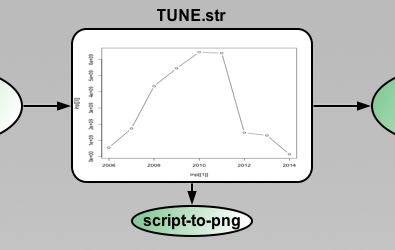
As example we can study how to make plots for some STR file. Imagine that you have some Resource with attached STR file:
This file: TUNE.str contains:
Streamz	1
Note	"Streamfile manufactured from user-specified data in file:RNB-Profiles-P10-P50.xls"
Note	"Case:P50"
Char	"BO+W"
Variable	Year	Integer
Variable	Group	String

Data

Set	Group	TUNE

Year	Amounts  SO	       SG	      SW
2006	         271552  555555550   13781
2007	         150029  1736142619   6788
2008	          26812  4347876676   1239
2009	         178500  5451284722	0
2010	        109233  6447013889	0
2011	         40767   6385229167	0
2012	        151500  1478472222    6122
2013	        135000  1305000000    5510
2014	         15000   145000000	     612
There is a table that can be easily loaded with "R" language. For generating graphic "Year" --> "Amounts", only 4 lines of "R" code is required:
The script file: str-to-png.r contains:
png("TUNE.str.png")
inp <- read.table("TUNE.str", sep="\t", skip=11, h=T)
plot(inp[[1]], inp[[2]], type="b")
dev.off()
Now you need to create simple script that calls this "R" script file and generates png
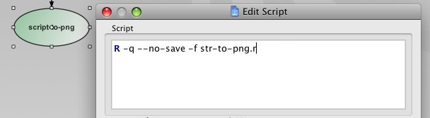
(You need to have "R" in your PATH environment variable)
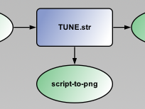
When you run the project you get TUNE.str.png. Which you can attach as background directly to your Resource file.
Then the plot will be generated each time your resource got new data and is completed during project run and background of the Resource will be updated automatically.
Actually you can attach the image to any other item - "script-to-png" or canvas background or background of composite or annotation - it does not matter, Pipe-It watch if the image is changed and updates appropriate items on canvas. You can create several "monitors" to watch how some diagrams are changed during run etc.
http://www.r-project.org/screenshots/screenshots.html
http://addictedtor.free.fr/graphiques/thumbs.php?sort=votes
The following file types are used by Pipe-It. The extensions are typical but not mandatory.
*.stz Streamz engine driver files
*.str Pipe-It resource (stream) files
*.psm Pipe-It utility driver files
*.log Log files containing messages logged by Streamz or utilities.
*.chr Characterization files containing the format description of resources
*.cnv Conversion files containing methods for conversion of resources from one format to another
*.ppm Logical project model in XML format
*.ppv Visualization of the project model in XML format
*.ppl Linkz library of the project in XML format
*.pps Streamz library of the project in XML format.
The program performs operations on a project depending on 3 required files:
Optionally, two additional files may be used for projects that are typical:
Copyright 2006, 2013 Petrostreamz AS. All rights reserved. No part of this manual may be reproduced, stored in a retrieval system, or translated in any form or by any means, electronic or mechanical, including photocopying and recording, without the prior written permission of Petrostreamz AS, Granaasveien 1, 7048 Trondheim, Norway.
Use of this product is governed by the License Agreement. Petrostreamz AS makes no warranties, express, implied, or statutory, with respect to the product described herein and disclaims without limitation any warranties of merchantability or fitness for a particular purpose. Petrostreamz AS reserves the right to revise the information in this manual at any time without notice.