The Optimizer is the interface for multiple launches of an entire Pipe-It project (or !subset/composite of a project) in an optimization context. It acts as a GUI control panel where it is possible to run the Pipe-It project automatically over and over again in a sequence of iterations utilizing a solver, or in single runs without solver, but still collecting History data. Optimization is also possible through Pipe-Itc, which runs from the command line without a GUI.
The purpose of optimization would typically be to let the computer find a combination of values of some selected input variables which optimize a specified output variable. The output to be optimized could be for example the amount of oil, the value in USD, or something else that the user has specified.
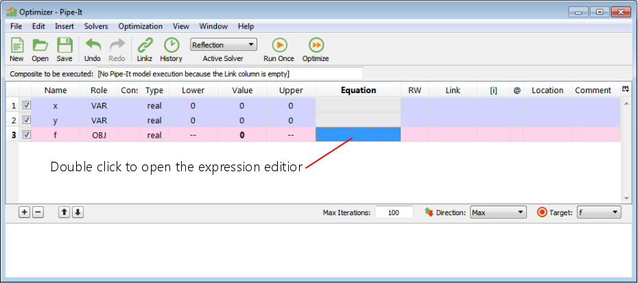
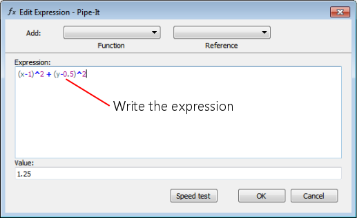
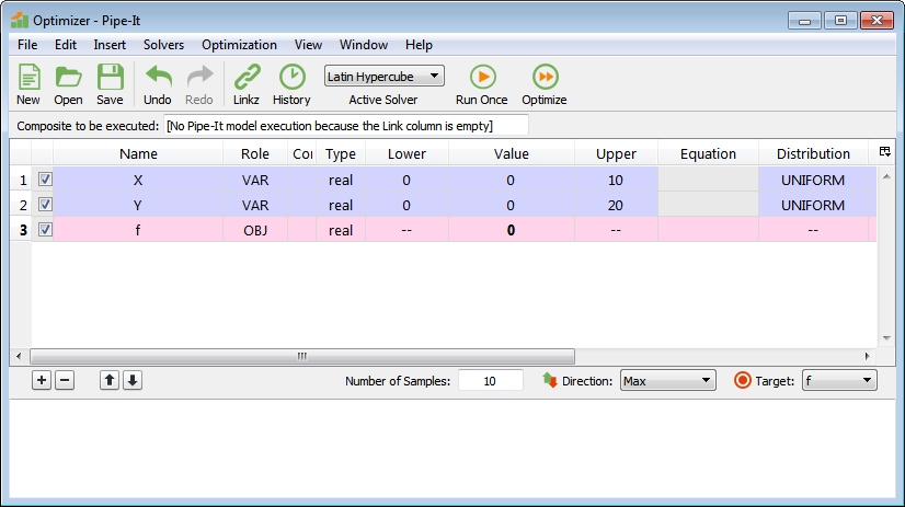
As a first example, to get to know the appearance of the optimizer and how to use it, we shall make an example to minimize the value of a function f(x,y) of two variables. Note that there is no Pipe-It project model with simulations involved in this simple example, only the function defined in the optimizer:
f(x,y) = (x-1)2 + (y-0.5)2
By inspection we can easily see that the solution is x = 1, y = 0.5, which gives the minimum value of f = 0.
Now start Pipe-It (not shown).
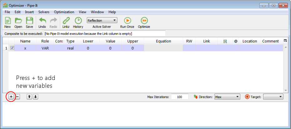
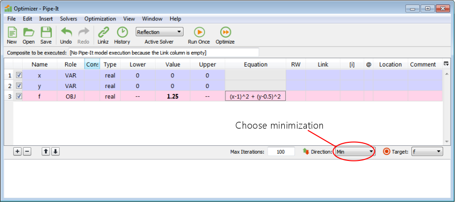
Press the ‘+’ button to add new variables. Add three variables.
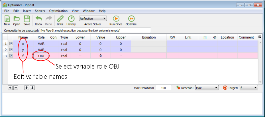
Double click on the variable names and write the names. Double click and select the variable role from a drop-down list. OBJ means objective function (which is to be optimized).
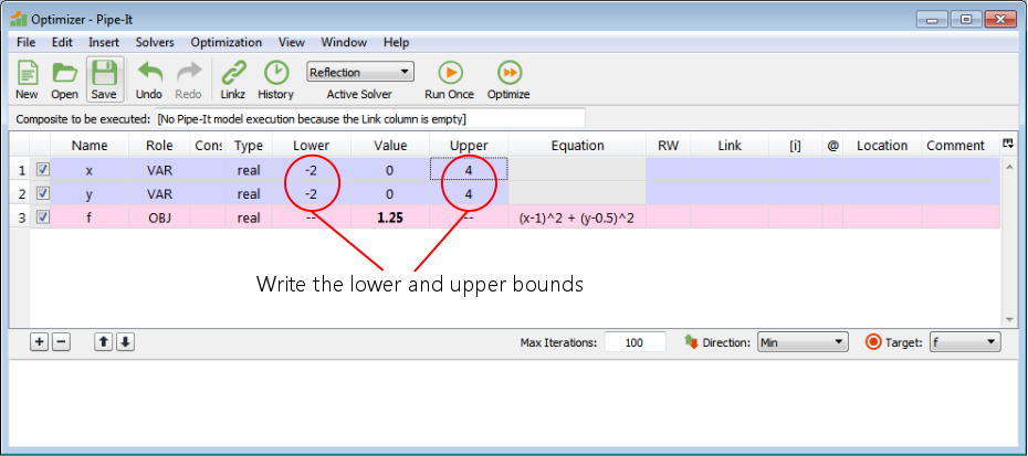
The lower and upper bounds that we write here are the bounds that the solver must stay within when it sets values for the decision variables. We have written that the solver must stay within [-2,4] for both variables in this example.
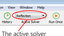
Select the solver that will be doing the optimization.
Now save the ppo file (not shown).
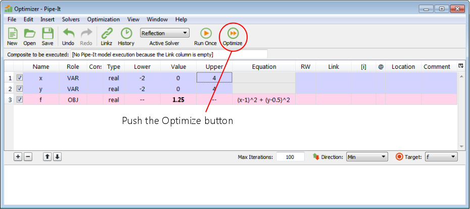
Push the Optimize button. This hands the execution control of the optimization over to the solver. Note that model execution in this simple example is just that the optimizer will evaluate the expression for f.
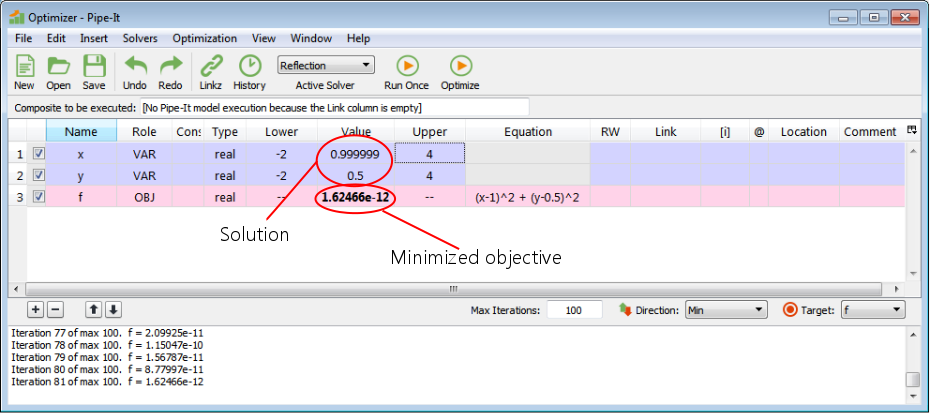
It found the solution x = 1, y = 0.5. The minimum value of f ~ 0.
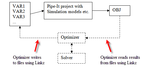
Schematic which shows informally some of the data and execution flow during optimization. The execution goes around and around in iterations.
During optimization, the algorithm and execution is controlled by the solver. Briefly explained, for each iteration the solver determines values for the decision variables and sets the values into the optimizer. The !optimizer/Pipe-It calculates auxiliary variables, writes data to files utilizing Linkz, executes the Pipe-It project, reads data from files utilizing Linkz, calculates more auxiliary variables and the objective and makes the values available to the solver. Then the solver uses the results in its solution algorithm and may start a new iteration with different values for the decision variables.
More information about this and the roles of the different variables can be found on Optimization Variable.
The execution of the numerical solver algorithm is done by a solver. Pipe-It offers a collection of different solvers that the user can choose from.
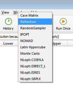
Drop-down menu for selection of solver. The figure shows the solvers that are currently provided with Pipe-It. Most of them are implemented in dynamic libraries (*.dll on Windows). The solver libraries are also known as solver plugins in the Pipe-It context. It is possible to add new solvers to Pipe-It by placing such plugin files in the Solvers folder in the Pipe-It installation folder. They will then immediately become available through this menu for use in Pipe-It. Note also that there can be more than one solver in each plugin.
The user can select which solver to use. The solver selection is saved in the ppo file. The solvers are documented in more detail as follows:
Pipe-It has an open Application Programming Interface (API) for solver plugins, which makes it possible for anyone to make their own solver plugins. The API is documented in detail in separate documents. As mentioned, when a plugin is placed in the Solvers folder in the Pipe-It folder, it becomes available immediately for use in Pipe-It. So, implementing a new solver and making it available for use in Pipe-it can be done without modifying the source code of Pipe-It.
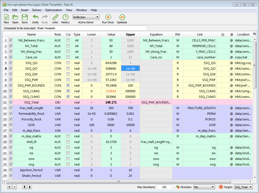
A more realistic optimizer case. Some things to notice: Only three of all the auxiliary variables have constraints switched on. Those that are off have had their cells for Lower and Upper emptied by the user and grayed out. VARs can not have expressions (grayed out cells), while CONs can not have expressions if they are connected to a link. Equation expressions are not shown in their entirety due to small cells, but by double clicking, they will be shown in the expression editor. In the Link column are listed the names of links defined in Linkz, which the variables are connected to. There are no links to arrays, so the [i] column is empty. Location shows the filenames of the data that are linked to. The case is set up to maximize the Net Present Value.
Variable 3 has constraints switched on. Due to its Role it will be calculated before the Pipe-It model execution. If it is calculated to be outside one of the bounds (i.e., violate the constraint), the model will be executed anyway because it is not until after the model execution in each iteration that the solver gets to know about the constraints violation.
Be aware of:
See Optimization Variables for more details.
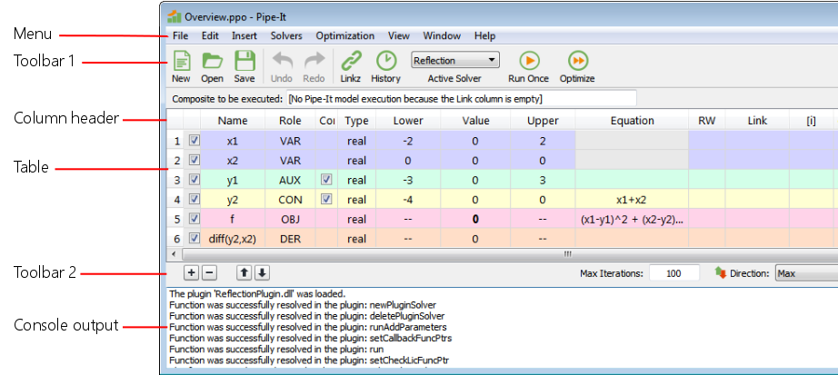
Overview of the Optimizer GUI. The parts listed on the left side of the figure are documented below, in a top to bottom sequence.
This is the main menu of the Optimizer window. The submenu items are explained below.
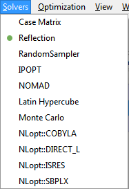
This menu shows the list of available solvers, which is the same list as in the Active Solver drop-down menu.

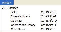
The window menu is identical to the Window menu in the main window.
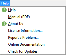
The help menu is identical to the Help menu in the main window.
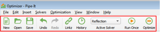
This is the first Optimizer toolbar. Many of these items are duplicating the functionality in the menus; in those cases there is a link to the explanation. The toolbar can be hidden by right-clicking on the toolbar, or the menu at the top, and unchecking Optimizer.
Column selection: Pressing this little icon opens a menu to select which columns are to be visible or hidden. The setting is saved automatically.
Column widths can be adjusted by dragging the heading separators. The column widths setting is saved automatically.
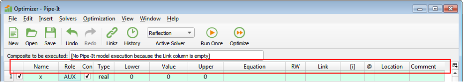
The table (see picture) shows the variables, one variable at each row. Each Role has its own background color. It is possible to select several rows by clicking and dragging in the vertical header (the line numbers on the left side), and several cells can be selected within the table. By holding down Ctrl, cells can be selected and deselected, thereby adding and removing cells in a selection. Clicking outside of a selected area changes the selection to that single cell, and the work continues on that cell. There are some different context menus available by right-clicking. Some cells must be double-clicked to be edited, others can be edited by writing directly. For numeric values, tool-tips (let the pointer stay on a cell) will show the full stored precision of the number. There are tool-tips on various other columns as well.
All operations, except Hide, done on elements in the table are covered by Undo and Redo. There is one limitation to the undo completeness: Values in the Value column produced by optimization or Run Once are not covered by undo. This means that Undo will recover the second last user edited value, and subsequent Redo will recover the last user edited value, not the execution result.
If Lower is greater than Upper, the numbers will be shown in red color.
If Value is out of bounds [Lower, Upper], it will be shown in red color.
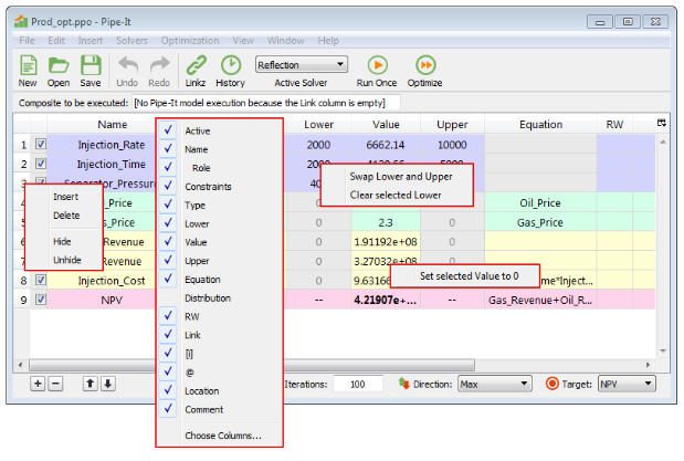
Context menus appear after right-clicking (on Windows). Which menu that appears depends on where the right-click was done. The figure shows the available context menus in the Optimizer.

Add decision variable, Delete selected variables, Move selected variables up, Move selected variables down.

Iteration output, warnings and error messages etc. are printed in the console window. During a run, if the output is scrolling rapidly due to much output, the user can click in the output text in the console window to stop the automatic scrolling and scroll up to the desired place (while new output is being added at the end, outside of the view). To restart the automatic scrolling one can scroll all the way down to the bottom and click below the output, or click in the console window and press Ctrl+End.
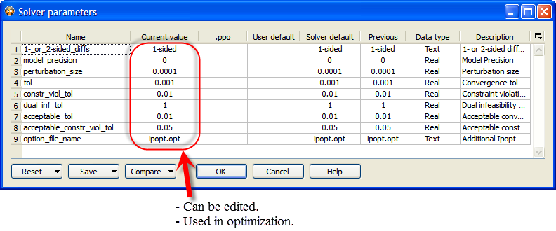
The figure shows the Solver parameters window with the parameters of
IPOPT as an example.
Each solver (e.g., IPOPT, Reflection, ...) defines its own set of parameters. The parameters' names and default values are transferred automatically from all the solvers to the optimizer so that they can be shown in this window. At any one time, the window shows the parameters of only the "active solver", as selected in the optimizer window (before the parameters window is opened).
Here is an explanation of the columns:
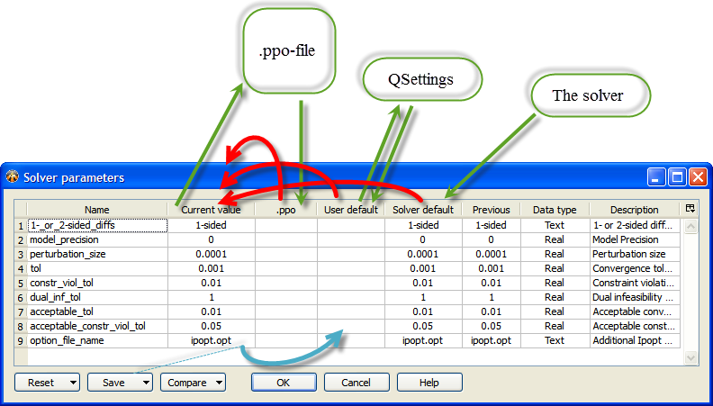
The arrows in the figure show the data flow of solver parameter values. Green arrows show the reading and writing of data. Red arrows show the initialization of the Current value column. Blue arrow shows the Save button action.
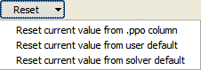
Copies the values from the columns mentioned in the different menu items to the Current value. (Red arrows in the figure).
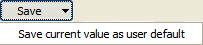
Copies the values of the Current value column to the User default column so that the values can be automatically saved in the QSettings. (Blue arrow in the figure).
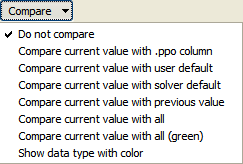
Compares the values in the Current value with other columns according to menu selection. Comparison results are shown as background color. Emphasis is on showing differences, and yellow means different values. The mode "Compare current value with all (green)" is different from the modes above in that the emphasis is on showing equality. It shows equality with green color, and if there is at least one column that is different from Current, it shows current in yellow (and no color on those that are different). (Try it out, it makes sense.)
The Help button shows a description of the active solver.
There is a context-menu on the right end of the header to hide columns, the same menu can also be opened by right-clicking on the column headers. Column widths can be adjusted by dragging the column separators in the heading. The hiding of columns and column widths are saved and restored automatically (in QSettings) between sessions. Row heights can be adjusted similarly to column widths, but are not saved and restored between sessions.
VAR: User- or optimizer-specified. May be written to file. Updated before any other variable and before model execution.
AUX: Either set by equation, read from file, or user-specified, in that order of priority. If set by equation, may also be written to file. Updated after VARs but before model execution.
CON: Unless a user-specified constant, either read from file or set by equation, after model execution. (Note: Constraints are recognized for all variables, not just the results labeled CON).
OBJ: Same as CON, except the optimizer will try to minimize or maximize it.
Before each model run (which could be an optimization iteration), all VARs are updated first. They will have either been manually specified by the user, or else set to new values by the optimizer engine. VARs are never set by equation. If a VAR is associated with a file, it will be written to its file during this update phase.
Then, still before the model run, each AUX variable will be updated in turn. An AUX may be associated with an equation, a file, both, or neither. If it has an equation, it will always be set by that equation (using the current values of any referenced variables). If it also has a file, the updated value will then be written to the file. If it has a file but no equation, then it will be read from (instead of written to) that file. If it has neither equation nor file, it will just be used as a user-specified constant.
After the VARs and AUXs have been updated and (if necessary) written to their files, the model will then be executed.
After the model execution, all other variables (CON and OBJ) will be updated in the order specified, regardless of type. Each of these variables can have either an equation or a file, but not both (it can also have neither, which would just make it a user-specified constant). If it's not just a constant, then it will either be set from its equation (using the current values of any referenced variables) or read from its file.
Constraints will then be tested for all variable types (not just CON, which is now really a misnomer) and fed back, along with the OBJ, to the optimizer (if necessary).
Some solvers are provided with the default installation of Pipe-It. They are described below.
This solver is intended to provide a succession of random values (within the defined Lower and Upper bounds) of the VAR variables defined in the Optimzer and launch the project with those values. The values of OBJ and CON are read after the completion of run and stored as part of the optimization History. The number of iterations will depend on the Max Iterations value. At the end of all the iterations, the best solution will be restored. This solver is ideal for getting a feel of the solution space and is often the first step in an optimization problem.
Random Sampler can run also when there is no OBJ variable defined.
Case matrix is different from the other solvers in that it provides a spreadsheet to the user to enter the values with which to run the project. (In older versions of Pipe-It the Case Matrix is referred to as Experimental Design.) The project can then be executed for any row (set of values) or for all the cases. The values of OBJ and CONS are read after the completion of the run(s) and stored in the History records. Cut and paste from Excel into the Case Matrix is possible. The case matrix can be saved as a tab-delimited file. Case Matrix can typically be used for performing scenario studies and evaluating the performance of the project for sets of input variables. (Case matrix is built-in and not in a plugin.)
The Nelder and Mead (1965) reflection simplex algorithm is the default "real" solver provided with Pipe-It. This algorithm does not require derivatives and is very robust. It utilizes a direct search method of optimization that works moderately well for stochastic problems. It is based on evaluating a function at the vertices of a simplex, then iteratively shrinking the simplex as better points are found until some desired bound is obtained. Lagarias et al. (1998) studied the convergience properties of the Nelder-Mead reflection simplex, and concludes that they are at best linear.
The Reflection solver allows specification of two parameters that affect the convergence of this solver:
Fractional Convergence Tolerance (ftol): the solver converges if the absolute value of the difference between the best and worst objective values within the current simplex (including penalties for constraint violations) is less than or equal to ftol times the absolute value of the best objective value. This tolerance determines the accuracy to which the optimum objective can be found, but it should be kept larger than the precision (i.e., noise or round-off level) of the model. Otherwise, before converging, the algorithm could encounter conflicting directional trends, which could lead to expansions of the simplex before the second convergence criterion (below) could be met. The current default (5e-7) is intended to give 6 digits of accuracy in the optimum objective, but it probably requires at least 7 digits of precision in the model.
Movelength Convergence Tolerance (ltol): the solver converges if the simplex contracts to where the best vertex is less than or equal to the square root of ltol in distance from any other vertex (with the distance between the upper and lower bound for any independent variable defined as 1). This tolerance determines the accuracy to which the independent variables at the optimum solution can be found, but it should be kept larger than the minimum relative change in the independent variables that would produce a measurable change (greater than the noise level) in the objective. Unfortunately, this is a little difficult to estimate without prior knowledge of the second derivatives of the objective at the optimum solution. The current default (1e-12) is intended to determine the independent variables to within 1e-6 times the differences between their bounds, which might be a higher accuracy than many problems warrant.
The solver converges if either criterion is met.
TIP: If the defaults don't seem to work well for a particular problem, and the precision of the problem is estimated to be epsilon, say, then one might try setting ftol to somewhere between 10 and 100 times epsilon and ltol to roughly ftol squared.
http://en.wikipedia.org/wiki/Nelder-Mead_method
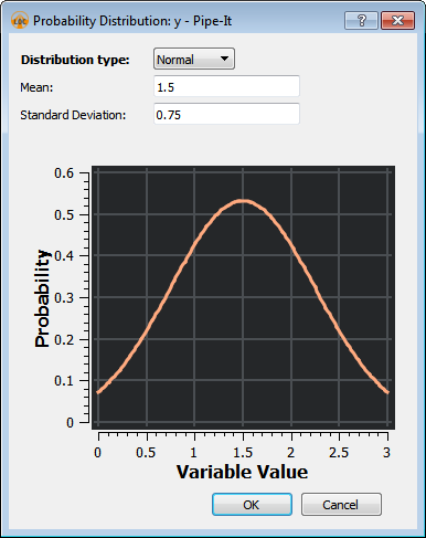
The Monte Carlo sampling method (also referred to as "Monte Carlo Simulation") is a random sampling method that chooses variable sampling points according to probability distributions associated with each variable.
When Monte Carlo is selected from the Active Solver drop-down, a new column "Distribution" appears in the variable table:
By double-clicking on the cells in the Distribution column, a new dialog appears where the probability distribution for the Variable can be specified:
Latin hypercube sampling is a type of Experimental Design. It is a statistical method for generating a sample of plausible collections of parameter values from a multidimensional distribution. The sampling method ensures than each variable is sampled evenly according to the variables probability distribution. Probability distributions are assigned to each Variable in the same manner as described for the Monte Carlo Sampler.
The Latin Hypercube Sampler is useful for generating a limited number of model runs that span the entire solution space as well as possible.
For a simple optimization case containing two variables, X and Y:
The Latin Hypercube algorithm will generate 10 combinations of variable values to execute the model on. The variable values will be selected such that:
Latin Hypercube samples may be generated as shown below:
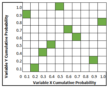
Where green squares indicate an interval a sample will randomly be selected from.
IPOPT, short for "Interior Point OPTimizer, pronounced I-P-Opt", is a software library for large scale nonlinear optimization of continuous systems. This is the default derivatives-based solver provided with Pipe-It.
The following parameters can be adjusted:
Plugin parameters
1- or 2-sided differences: Specifies whether the numerical differentiation should be 1- or 2-sided.
Model precision: If set to a value larger than 0, it will be used to automatically set the perturbation size, the convergence tolerances and the constraint violation tolerances in the following ways:
Perturbation size will be the square root of the model precision.
Convergence tolerance and constraint violation tolerance will be the square root of the perturbation size.
Acceptable convergence tolerance and acceptable constraint violation tolerance will be 5 times the value of convergence tolerance and constraint violation tolerance.
Perturbation size: Perturbation used in numerical differentiation.
Max step size: Maximum change in variable values between iterations. Input as a fraction of the distance between the upper and lower bounds. Allowed values are between 1e-10 - 1.0.
IPOPT solver parameters
Convergence tolerance (tol): See link
Constraint violation tolerance (constr_viol_tol): See link
Dual infeasibility tolerance (dual_inf_tol): See link
Acceptable convergence tolerance (acceptable_tol): See link
Acceptable constraint violation tolerance (acceptable_constr_viol_tol): See link
Additional Ipopt options file (option_file_name): The file name of the file where additional parameters for the IPOPT solver can be set. A list of the most common options can be seen in the IPOPT Options Reference.
Explanation of the difference between tolerances and acceptable tolerances from the IPOPT documentation for acceptable convergence tolerance:
There are two levels of termination criteria. If the usual "desired" tolerances (see tol, dual_inf_tol etc) are satisfied at an iteration, the algorithm immediately terminates with a success message. On the other hand, if the algorithm encounters "acceptable_iter" many iterations in a row that are considered "acceptable", it will terminate before the desired convergence tolerance is met. This is useful in cases where the algorithm might not be able to achieve the "desired" level of accuracy.
http://www.coin-or.org/projects/
NOMAD (Nonlinear Optimization by Mesh Adaptive Direct Search) is
a C++ implementation of the Mesh Adaptive Direct Search (Mads)
algorithm. http://www.gerad.ca/nomad/Project/Home.html
This solver can be used for mixed-integer nonlinear problems.
NLopt is an open-source library for nonlinear optimization, providing a common interface for a number of different free optimization routines available online as well as original implementations of various other algorithms.
A selection of the NLopt algorithms are made available in Pipe-It.
COBYLA: An algorithm for derivative-free optimization with nonlinear inequality and equality constraints.
ISRES: An evolutionary strategy algorithm for nonlinearly-constrained global optimization (or at least semi-global; although it has heuristics to escape local optima). The evolution strategy is based on a combination of a mutation rule (with a log-normal step-size update and exponential smoothing) and differential variation (a Nelder–Mead-like update rule). The fitness ranking is simply via the objective function for problems without nonlinear constraints, but when nonlinear constraints are included the stochastic ranking proposed by Runarsson and Yao is employed. The population size for ISRES defaults to 20×(n+1) in n dimensions.
DIRECT-L: A global deterministic-search algorithm based on systematic division of the search domain into smaller and smaller hyper rectangles.
SBPLX: A variant of Nelder-Mead that uses Nelder-Mead on a sequence of subspaces. Is claimed to be much more efficient and robust than the original Nelder-Mead, while retaining the latter's facility with discontinuous objectives
http://ab-initio.mit.edu/wiki/index.php/NLopt
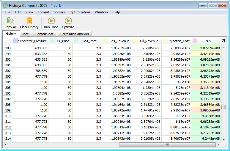
The history window contains information on previously executed model runs. All model runs started from the Optimizer are stored in the history window, both when run as part of an optimization, and when run by pressing "Run Once". The window is organized into four tabs:
History: A table of parameter values for previous model runs.
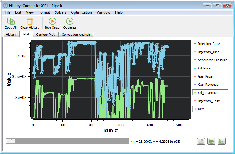
Plot: Plotting of the optimization history.
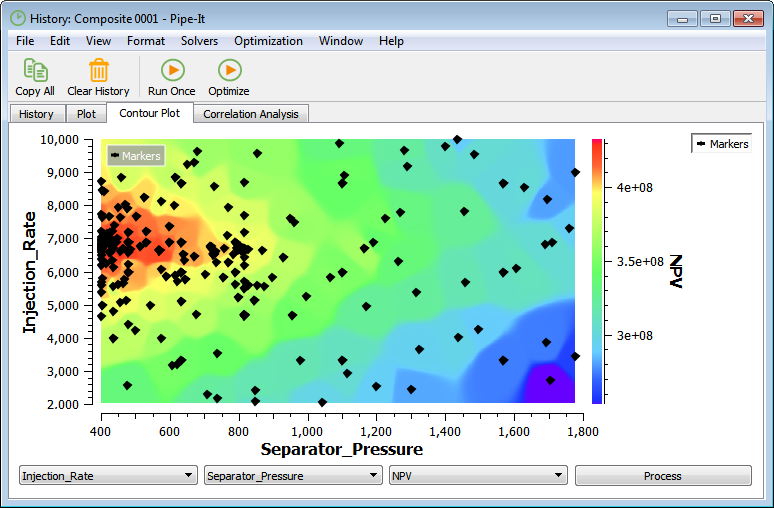
Contour Plot: Surface plots of two VARs against an OBJ or CON parameter.
Correlation Analysis: Linear correlation between a VAR and an OBJ or CON.
The table in the History tab contains variable values for previous model runs together with information on when the model was executed, the type of solver used, and if the model executed successfully.
In the Plot tab it is possible to plot the optimization history. The optimization parameters you want to show in the plot can be selected by clicking on the right-side legend.
The Contour Plot tab features a surface plot of two VARs against an OBJ or CON. The VAR values are plotted against the x- and y-axis, while the OBJ or CON values are represented by a color range. Interpolation is used to estimate OBJ or CON values between sample points.
The variables to base the contour plot on are selected from the three drop-down menus. By pressing "Process", the contour plot is generated. This may take several seconds, depending on the number of historical runs.
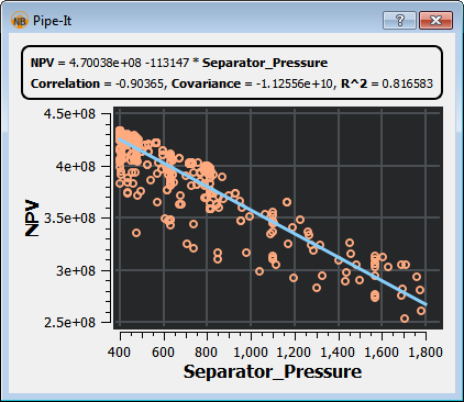
In the Correlation Analysis tab, a table of correlation parameters between VARs, OBJs and CONs are presented. The correlation parameter indicates how well two parameters correlate linearly. The correlation parameter can have values between 1.0 and -1.0, where a positive number indicates positive correlation, and a negative number indicates inverse correlation.
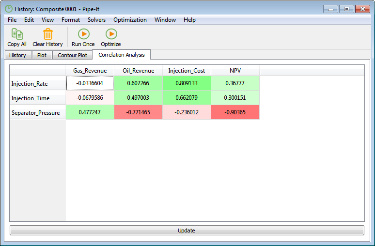
By double-clicking any of the cells in the table, a cross-plot of the two corresponding optimization parameters are shown. The plot includes a linear curve fit of the two parameters.
Active Solver
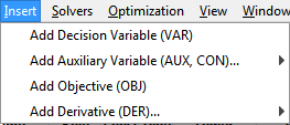
Add Auxiliary Variable...
Add Decision Variable
Add Derivative...
Add Objective
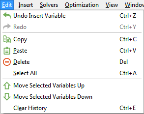
Clear History
Close
Copy
Cut
Delete
Direction
Edit Menu
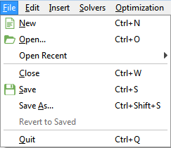
File Menu
Help Menu
History
Insert Menu
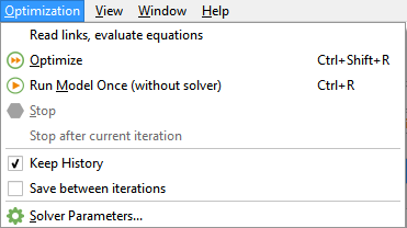
Keep History
Linkz
Max Iterations
Move Selected Variables Down
Move Selected Variables Up
New
Open Recent >
Open...
Optimization Menu
Optimize
Paste
Precision
Quit
Redo
Revert to Saved
Run Model Once (without solver)
Save As...
Save
Save and Plot...
Save between iterations
Select All
Solvers Menu
Solver Parameters...
Stop
Stop after current iteration
Target
Undo
View Menu
Window Menu