Streamz is built to take instructions from a user written driver file using the Streamz command "language". The user typically states fluid characterizations, specifies conversions among multiple characterisations and causes the program to convert quantities contained in stream files containing hundreds (or millions) of streams. A rich set of about 30 commands (primary keywords) are understood by Streamz (but not very well by users). The alphabetical list is given below. Each is explained, with examples on page linked to the command.
Primary Keywords Brief Description BIPS Enter a table of Binary Interaction Parameters CD Change Directory CHARACTERIZATION Name and enter a fluid characterization CLEAR Clear named filters and streams COMBINE Combine input streams into named streams COMPONENT Enter a table of properties for current characterization CONVERT Define a conversion procedure from a named to "current" characterization COPY Copy streams from input to output stream files DEFINE Define named filters DOMAIN Name domains and their types ECHO Turn on echoing of input (driver) files END Declare the end of current primary keyword EOF Declare the end of file EOS Declare the Equation of State for next characterization FILTER Define named filters GAMMAFILE Open and close files for Gamma distribution results INCLUDE Include files LUMP Create lumped fraction from defined components MIX Prepare named streams from other streams or components PROCESS Process a stream through a set of connected separators REDUCE Convert from molar streams to volumetric streams RESTORE Make a previously defined characterization "current" SEPARATOR Define a separator SPLITFILE Open and close split files STREAMFILE Open and close stream files TABS Define "tab" positions for current file TAG Add variables & values to named streams TABULATE Sum-up and tabulate variables while converting TITLE Define a boxed title TOTAL Sum named streams VARIABLE Name variables and their types WRITE Output named streams to stream file(s)
ALIAS Table: It is a list of Aliases of Primary Keywords and their Sub-Keywords.
(see also: ALIAS Table for alternative keywords)
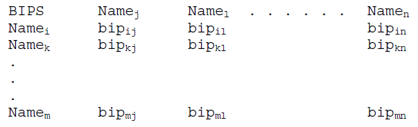
The BIPS keyword initiates the tabular input of the binary interaction parameters. The arguments (Name1 Name2 etc.) following this keyword are predefined component names (in any order). Following this command line, the program expects a formatted table containing the values of binary interaction parameters, where the values “line up” (see: line up procedure ) with their heading, as shown below:
Here, for example, Namei is the name of the component i, as specified in the property table, and bipij is the parameter for the binary interaction of components i and j. A blank line or the word END completes a binary interaction parameter table. Any of the table entries may be left blank (defaulting to a previously specified value, initially zero). Specifying a value for bipij will also specify the same value for bipij. Any attempt to specify a non-zero bipii will be ignored.
For associating components to a bipij value, the component name for i is taken as the first entry in the row, and the component name for j is found using the table line up procedure described here. This strategy allows the use of blanks within the table, wherever default entries are desired, without causing the rest of the table to become misaligned.
The entry of BIPS could be spread out into multiple tables, for example, if a single table was too wide for the user’s preference (or the editor’s).
Example 1: Single BIPS table.
BIPS			  CIN2	      CO2C2	     C3-6      C7-9F1-2	      F3-8	      F9
CIN2	                0.0000	   5.74E-02      4.13E-04      2.72E-04   2.72E-04      2.72E-04
CO2C2      	      5.74E-02	     0.0000      5.75E-02      4.79E-02   4.79E-02      4.79E-02
C3-6	      	      4.13E-04     5.75E-02        0.0000        0.0000	    0.0000        0.0000
C7-9F1-2  	      2.72E-04     4.79E-02        0.0000        0.0000	    0.0000        0.0000
F3-8		      2.72E-04     4.79E-02        0.0000        0.0000	    0.0000        0.0000
F9		      2.72E-04     4.79E-02        0.0000        0.0000	    0.0000        0.0000
END
Example 2: Complete BIPS definition spread over multiple tables, with some entries in the last table left empty, and defaulting to 0.0.
BIPS	    N2	         CO2	    C1	          C2          C3	 IC4	      C4         IC5
N2	0.0000	      0.0000	0.0250	      0.0100      0.0900      0.0950      0.0950      0.1000
CO2	0.0000	      0.0000	0.1050	      0.1300      0.1250      0.1200      0.1150      0.1150
C1	0.0250	      0.1050	0.0000	      0.8260     -0.1120      0.0265      0.0000      0.0000
C2	0.1000	      0.1300	0.0826	      0.0000      0.0130      0.0170      0.0000      0.0000
C3	0.0900	      0.1250   -0.1120        0.0130      0.0000      0.0200      0.0000      0.0000
IC4	0.0950	      0.1200	0.0265	      0.0170      0.0200      0.0000      0.0149      0.0000
C4	0.0950	      0.1150	0.0000	      0.0000      0.0000      0.0149      0.0000      0.0129
IC5	0.1000	      0.1150	0.0000	      0.0000      0.0000      0.0000      0.0129      0.0000

BIPS	    N2	         CO2	    C1	          C2 	      C3	 IC4	      C4	 IC5
C6	0.1100	      0.1150	0.0000					                      0.0120
F1	0.1100	      0.1150	0.0014					                      0.0000
F2	0.1100	      0.1150	0.0019					                      0.0000
F3	0.1100	      0.1150	0.0027					                      0.0000

BIPS	    C5	          C6        F1	          F2	      F3
N2	0.1100	      0.1100	0.1100	      0.1100      0.1100
CO2	0.1150	      0.1150	0.1150	      0.1150	  0.1150
C1	0.0000	      0.0000	0.0014	      0.0019	  0.0027
C2
C3
IC4
C4
IC5		      0.0120	0.0000	      0.0000	  0.0000
C5		      0.0000			          0.0000
C6		      0.0000	0.0037	      0.0000	  0.0000
F1		      0.0037	0.0000	     -0.1280     -0.2000
F2		      0.0000    0.1280        0.0000	  0.0000
F3		      0.0000    0.2000        0.0000	  0.0000
The EOS property table consists of a row of heading, a possible row of units, and rows of component values. A component value is associated with a heading according to its line up.
Columns are defined by headings in the first row of a table. Subsequent lines contain table entries or values that are associated with a column in the following logic:
b) If a heading is not intersected, move left on the heading row until a heading is intersected.
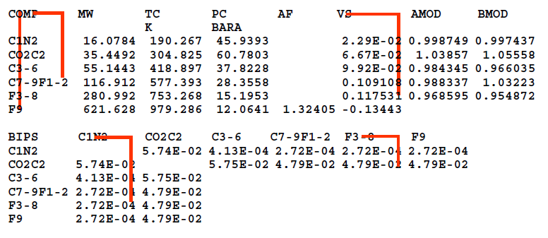
For the BIPS table and associating components to a kij value, the component name for i is taken as the first entry in the row, and the component name j is found using the table line up procedure described above.
Example of Table Line Up
The CD keyword allows the user to change the current directory for inclusion of files or to open files from certain directories, without the need to specify the path along with the name of file. This keyword provides the functionality of the change directory command of many OSes.
path_spec may include symbols typically used in “change directory” commands of supported OSes (Win9x/NT, DOS, Unix, Max OS) like,
“.” for current directory,
“. .” for parent directory,
“/” (or “\” or “:” depending on the OS) for directory name separators.
If the path_spec includes embedded spaces, it should be enclosed within quotes. Care should be taken while using these special symbols, as they may trigger errors if used on the wrong OS.
Example 1: Relative path specification on DOS/Windows
CD `..\..\InputFiles\BaseCase`
In this example the current directory is change to BaseCase under InputFiles, which is one level above the previous current directory.
Example 2: Absolute path specification on DOS/Windows
CD `D:\Data\BaseCase`
In this example the current directory is changed to BaseCase under Data, which is under the root directory on drive D.
Example 3: Absolute path specification on Unix
CD `~/Simulation/Sensitivity/EOS6`
In this example the current directory is changed to Sensitivity under Simulation, which is under the user’s login directory.
(see also: ALIAS Table for alternative keywords)
The CHARACTERIZATION keyword specifies a name for the characterization which is being described. The argument char_name makes it a named characterization. The actual description of the characterization is done using the CHARACTERIZATION and the BIPS keywords. The CHARACTERIZATION keyword makes the named characterization "current" and associates the property table (COMP keyword) and the binary interaction parameters (BIPS keyword) with it.
This named characterization is also used in a CONVERT keyword which defines the conversion between two characterizations. The RESTORE keyword can be used later in the same file to change back to a previously defined characterization if another characterization has been defined subsequently (see Example 2)
If the argument char_name includes embedded spaces, it should be enclosed within quotes (see Example 1). Otherwise, no quotes are required (see Example 2).
Example 1: Use of keyword; char_name includes embedded spaces
CHAR `EOS15 Gas Cap`
In this example, the EOS properties and BIPS that is supposed to be entered after this command are stored with the characterization name “EOS15 Gas Cap”.
Example 2: Use of alternate keywords (see ALIAS Table); No quotes needed for char_name since it does not include embedded spaces
CHARACTERIZATION EOS3Comp
COMP	MW
C1	44
C4	78
C10	200

PROPERTIES AnotherChar
COMP	MW
C1	44
C2	56
.	.
.	.
.	.
F3	256
F4	316
F5	478

RESTORE EOS3Comp
In the above example, a characterization named EOS3Comp is defined and then AnotherChar is defined making it the current characterization. To make EOS3Comp "current" again, a RESTORE command has to be used.
This keyword is used to CLEAR all the FILTERS and named STREAMS from the memory. When used with optional sub-keywords it can also CLEAR either one or the other. When filters are defined, each new filter is stored in memory, even if the new one has a name the same as a previous one. This is because the definition of the new filter itself may use the old one. In this way, each new use of the FILTER command stores the filter and its logic in memory. This way it is available for use in any command such as COPY, COMBINE etc.
Similarly, each use of the COMBINE (or TOTAL) command stores the named STREAMS and all its associated variables and amounts in memory. To generate proper output for some applications, like a reservoir simulator, the number of FILTER and COMBINE commands may run into hundreds. The processing of such streams may take unacceptable duration. To solve such problems, frequently used FILTER and COMBINE commands can be used repeatedly. To make such processing efficient, the un-required filters and/or streams may be erased from memory using the CLEAR command.
Example 1: Various uses of CLEAR command
.
.
.
CLEAR Filters
.
.
.
CLEAR Streams
.
.
.
CLEAR
This example illustrates the various possible uses of the CLEAR keyword. It first clears all the filters, then clears all the streams in memory and then clears both.
(see also: ALIAS Table for alternative keywords)
COMBINE stream_nickname
[IF filter_name]
[WEIGHT [BY|OVER] var_spec [AND var_spec ]…]
[OVER var_spec [AND var_spec ]…]
[NORMALIZE]
[SCALE value]
This keyword allows the aggregation of streams satisfying filter criteria (or named filters using the FILTER command) into new named streams with the name stream_nickname. The COMBINE command creates a named stream by aggregating input streams based on named filters and other options. The first argument to this command is the name of the resulting combined stream. Multiple arguments can follow, each either a named filter or other manipulative option. A COMBINE command does not initiate writing to a file; this is accomplished with a corresponding WRITE command.
| Sub-Keywords | ALIAS |
| IF | |
| NORMALIZE | NORM |
| SCALING | SCALE, SCAL |
| AND | |
| WEIGHTING | WEIGHT, WEIGH |
| OVERING | OVER |
| WEIGHT OVER |
This keyword must be followed by the name of an earlier defined filter and results in the input stream being processed through it before being converted and combined. Only a single IF with its associated filter name is expected. If multiple occurrences are encountered only the last one will be used.
This keyword results in conversion of amounts of the output stream into fractions. If the input stream is in molar quantities, the output will be in molar fractions.
SCALING multiplies the output streams by a factor. This can be used for conversion from one set of units (e.g. moles/day) to another (moles/hour) if the output streams are required in a particular unit by the program using it. If SCALE 100 is used with the NORMALIZE command, the output streams are written in percentage instead of fractions.
It is used to specify multiple var_spec to the WEIGHT and OVER options. var_spec is the name of a numerical variable or domain, followed by its desired units, if applicable.
The WEIGHT option to the COMBINE command applies a product of the weigh variables to each converted stream after normalization (if requested). Each stream is then summed and multiplied by the value of SCALE (if used) to give the final stream. The argument to this command is one or more variables or domains (including units if applicable). Multiple weigh variables must be separated by the AND keyword. An optional BY keyword is allowed if the name of the weigh variable happens to be ‘over’.
The OVER option to the COMBINE command divides the converted and normalized (if requested) stream by a summation of the individual stream which have been multiplied individually by the product of the over variables. The argument to this command is one or more numeric variables or domains (including units if applicable). Multiple over variables must be separated by the AND keyword.
It is also possible to use the OVER keyword in conjunction with the WEIGHT keyword to mean a combined WEIGHT OVER options using the same variables for both options. This is a typical usage of these options when portions of the original stream are affected due to use of the FILTER command. The use of the WEIGHT OVER options in the COMBINE command needs to be explained in detail. The converted and normalized (if requested) streams are combined by the formula:
Final_Stream = Scale*Sum(Product(Weight-Vars)*Stream)/Sum(Product(Over- Vars))
Division by zero will never occur. If the denominator turns out to be zero, the final stream will be set to zero.
A "Weight-Var" is the value of a variable or the size of a domain (upper variable minus lower variable) requested by the WEIGHT option. The values or sizes are calculated in their requested units (if applicable) before any variables might be altered by filtering. This allows rates to be converted correctly to cumulative amounts, for example. Any undefined Weight-Var is assumed to be zero.
An "Over-Var" is the value of a variable or the size of a domain (upper variable minus lower variable) requested by the OVER option. Variable values are calculated in their requested units (if applicable) before any variables might be altered by filtering, but domain sizes are calculated in their requested units (if applicable) after the COMBINE command's filter has altered any necessary variables. This allows cumulative amounts to be converted correctly to rates, for example. Any undefined Over-Var is assumed to be zero.
Example 1: Simple use of COMBINE with single FILTER
COMBINE YEAR1: IF YEAR1
In this example, a named stream called “YEAR1” is created in memory. All streams satisfying the previous defined filter, also called “YEAR1” are converted and added to this named stream. The formula reduces to:
Final_Stream = Sum(Stream)
Example 2: Advanced use of COMBINE with FILTER, DEFINE, and WEIGHT OVER.
DOMAIN TIME T1 T2
DEFINE T1 0.0
DEFINE T2 1.0
FILTER YEAR: TIME GE ?T1? YEARS AND TIME LE ?T2? YEARS
COMBINE YEARS_?T1?-?T2? IF YEAR, WEIGHTING OVER TIME (DAYS)
This example assumes that "TIME" variables 'T1' and 'T2' are associated with each stream. It declares a DOMAIN called “TIME” made up of 'T1' and 'T2'. It then associates the wildcards 'T1' and 'T2' with the string 0.0 and 1.0 respectively. A filter called “YEAR” is defined with the criteria as the interval 0.0-1.0 years. A named stream called “YEARS_0.0-1.0” is created in memory. All streams satisfying the previous defined filter called “YEAR1” are converted and added to this named stream. Before adding, the domain "TIME"for the “current” input stream (i.e. T2 –T1 for this stream) is calculated and multiplies each stream quantity. After adding, the requested domain (i.e. the domain of the resulting stream) is calculated and divides the summed stream. This gives us back rates after starting with rates. The formula applied is:
Final_Stream = Sum(TIME domain for each stream before filtering) *Stream) / Sum(TIME domain after filtering)
Example 3: Weighted sum of streams
COMBINE SUMMED WEIGHTING BY FACTOR
This example assumes that a real variable “FACTOR” is associated with each stream. The streams themselves are in different molar units known to the user and the value of “FACTOR” reflects the unit conversion to a consistent set. The COMBINE command creates a total stream named “SUMMED”, converting the units to a consistent set. It is basically doing a weighted sum. The formula reduces to:
Final_Stream = Sum(Factor*Stream)
Example 4: Simple arithmatic average of streams
VARIABLE ONE INT
SET ONE = 1
COMBINE AVE WEIGHTING OVER ONE
This example declares an Integer Variable named “ONE” and SETs its value to 1 (any constant would do for this purpose). The COMBINE command creates an averaged stream named “AVE”, The WEIGH-vars and OVER-vars cancel out resulting in a simple arithmetic average. The formula reduces to:
Final_Stream = Sum(1*Stream)/Sum(1)
(see also: ALIAS Table for alternative keyword)
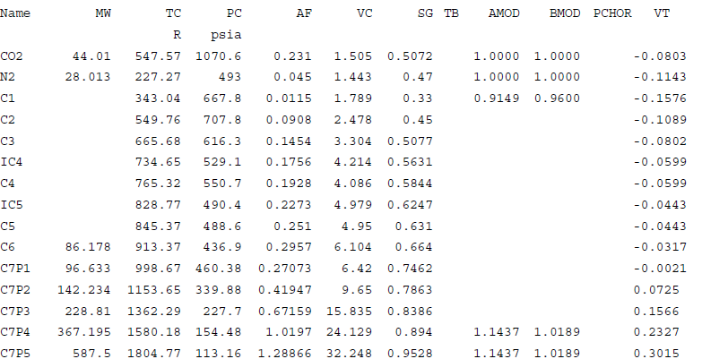
The COMPONENT primary keyword triggers tabular input of the full EOS property table that makes up the current characterization. The arguments (prop1 prop2 etc.) following this keyword are predefined critical properties for this characterization (in any order). This tabular input scheme is very flexible, allowing any of the component properties to be input in any order. Each property is identified by the heading keyword. For example, MW indicates molecular weight. The only constraint of the tabular input scheme is that any entries in the table that belong to a particular heading (i.e. property) should line up with the heading. This allows unknown entries to be left blank without misaligning the rest of the table.
The name of each component is listed under the COMPONENT heading. The value of any other property corresponding to that component is entered in the same row, lined up under the heading corresponding to the desired property. This input scheme is designed to enable cut-and-paste from any other data file or spreadsheet with minimal editing.
A possible row of units is allowed in the EOS property table immediately under the headings. If present, the units in that row are associated with the headings using the same line up procedure.
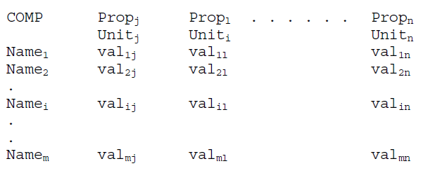
Here, for example, Namei is the name of component i, as specified in the property table, and valij is the value (entry) for the jth property of component i (identified by the heading Propj). A blank line or the word END completes a property table. Any of the table entries may be left blank (defaulting to a previously specified value, initially zero).
The entry of property tables could be spread out into multiple tables, for example if a single table was too wide for the user’s preference (or the editor’s).
Sub-Keywords ALIAS Brief Description MW Average Molecular Weight SG Specific Gravity TB Boiling Temperature LMW Lower Molecular Weight LSG Lower Specific gravity LTB Lower Boilling Temperature UMW Upper Molecular Weight USG Upper Specific Gravity UTB Upper Boiling Temperature TC TCR Critical Temperature PC PCR Critical Pressure ZC ZCR Critical Compressibility Factor VC VCR Critical Volume AF Acentric Factor VT VS Volume Translation AMOD A-parameter Modifier BMOD B-parameter Modifier VISZ VZ, ZCV Viscosity Z-factor PCHOR PARA Parachor Property FULL Full Name of Component END End of the Table ? or _ or ~ A comment to ignore a column
This is the average molecular weight property of a component. No units are associated with this property. The molecular weight of all the component as heavy as, or heavier than, the component specified to participate in Gamma distribution modeling, must be entered. Also, the input and output units (see CONVERT keyword) of MASS and MOLEs are considered compatible and internally convertible only if the MW property of the components are entered.
This is the specific gravity of a component. No units are associated with this property.
This is the boiling temperature of the component. The units of this property may be in any one of accepted temperature Units.
This is the lower molecular weight of the component. When discrete cuts of components (or fractions) are used in a characterization, this property identifies the lower bound of the cut-off molecular weight for the fraction. No units are associated with this property. This is particularly useful for specifying the bounds for discretization of a Gamma distribution model into ouput components. Specifying the average molecular weights (MW) in such cases, results in the bounds being average of them, thus giving rise to material balance errors.
This is the lower specific gravity of the component. When discrete cuts of components (or fractions) are used in a characterization, this property identifies the lower bound of the cut-off specific gravity for the fraction. No units are associated with this property.
This is the lower boiling temperature of the component. When discrete cuts of components (or fractions) are used in a characterization, this property identifies the lower bound of the cut-off boiling temperature for the fraction. The units of this property may be in any one of the accepted temperature Units.
This is the upper molecular weight of the component. When discrete cuts of components (or fractions) are used in a characterization, this property identifies the upper bound of the cut-off molecular weight for the fraction. No units are associated with this property. This is particularly useful for specifying the bounds for discretization of a Gamma distribution model into ouput components. Specifying the average molecular weights (MW) in such cases, results in the bounds being average of them, thus giving rise to material balance errors.
This is the upper specific gravity of the component. When discrete cuts of components (or fractions) are used in a characterization, this property identifies the upper bound of the cut-off specific gravity for the fraction. No units are associated with this property.
This is the upper boiling temperature of the component. When discrete cuts of components (or fractions) are used in a characterization, this property identifies the upper bound of the cut-off boiling temperature for the fraction. The units of this property may be in any one of the accepted temperature Units.
This is the critical temperature of the component. The units of this property may be in any one of the accepted temperature Units.
This is the critical pressure of the component. The units of this property may be in any one of the accepted pressure Units.
This is the critical compressibility factor (Z-factor) of the component. No units are associated with this property.
This is the critical volume of the component. Units of molar volume are acceptable using the acceptable units of volume and moles. These are listed under the the REDUCE keyword. An example would be M3/KGMOL.
This is the acentric factor of the component. It gives a measure of the steepness of the vapor pressure curve of pure components. No units are associated with this property.
This is the volume translation property of the component. Specifically, this is the dimensionless volume correction (si = ci/bi) used to improve the volume (density) prediction of 2-parameter Cubic EOSes, without affecting their VLE predictions, since it does not affect equilibrium calculations for pure components and mixtures. No units are associated with this property.
This is the A-parameter modifier of the component. It is a component dependent correction term for the EOS parameter A, to improve VLE predictions. No units are associated with this property
This is the B-parameter modifier of the component. It is a component dependent correction term for the EOS parameter B, to improve VLE predictions. No units are associated with this property.
This is the Viscosity Z-factor of the component. No units are associated with this property.
This is the parachor property of the component. It is a temperature independent parameter which is calculated experimentally and is proportional to the molecular weight of the component. It is used to calculate oil/gas interfacial tensions of complex hydrocarbon mixtures. No units are associated with this property.
This is the full name property of the component. No units are associated with this property. This property allows names including embedded spaces to be associated with a component (e.g. 'Carbon Dioxide'). This also allows remarks to be associated with components. Currently this is used to implement propriety names for an in-house process simulator.
This is sub-keyword signifies the end of the table of EOS properties.
Use of any one of these 3 special characters (_,?,~) directly in front of a table heading signifies a column comment. It basically results in the particular column (the heading and the respective 'lined up' data) being ignored by the program. This is useful if a user wants to temporarily not use some property of the characterization but retain it for reference only. Or if he/she wants to have 2 sets of a property, and use one while disabling the other.
The temperature and pressure units recognized in the EOS property table (also throughout the program) are:
Units ALIAS Description R RANKINE, RAN Rankine K KELVIN, KEL Kelvin F FAHRENHEIT, FAH Degree Fahrenheit C CELCIUS, CEL Degree Celcius ATMA ATM Atmospheres (absolute) ATMG Atmospheres (gauge) PSIA PSI Pounds per square inch (absolute) PSIG Pounds per square inch (gauge) BARA BAR Bar (absolute) BARG Bar (gauge) KPAA KPA Kilo Pascal (absolute) KPAG Kilo Pascal (gauge) MPAA MPA Mega Pascal (absolute) MPAG Mega Pascal (gauge) TORRA TORR Torr (absolute) TORRG Torr (gauge)
Example 1: Single property table, with units row.
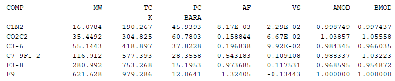
Example 2: Complete EOS property table with some entries left empty.
(see also: ALIAS Table for alternative keywords)
[WARNING [ON|OFF]]
[GAMMA inp_comp out_comp[FILE gamfil_nickname]
[IGNORE inp_comp]
[WEIGH inp_comp | AVERAGE|TOT [ w ] ]
[SHAPE [ parm_ini | parm_max | parm_min ]]
[BOUND [ parm_ini | parm_max | parm_min ]]
[AVERAGE [ parm_ini | parm_max | parm_min ]]
[ORIGIN | ZERO [ parm_ini | parm_max| parm_min ]] ][SET var_name var_value [ var_name var_value ]...]
[SPLITS splfil_nickname ]
[SPLIT | DELUMP in_comp [ out_comp spl_fctr [ out_comp spl_fctr ]...]]
This primary keyword defines completely the procedure to be used for conversions between a specified and the “current” characterizations, the units of input and output streams, and the quantity to be conserved in the conversion (if applicable).
Currently two procedures are available: 1) Gamma, and 2) Split.
The Gamma method is specified using the GAMMA sub-keyword. This method uses the Gamma distribution procedure to first fit the input stream to the Gamma model and then to calculate the amounts in the output stream corresponding to this calculated model.
The second method is to supply a set of split factors using the SPLIT sub-keyword. A combination of the two methods is also possible. This is usually the most typical procedure as the heptanes plus (C7+) components are best converted using the Gamma distribution and the hexanes minus (C6-) components are converted using split factors.
The first argument to the CONVERT keyword is the name of a defined characterization. The CONVERT command requires its first line to be of the form:
CONVERT input_char FROM in_units TO out_units CONSERVE cons_units
The above options must appear on the same line as the CONVERT keyword, and no other sub-keywords may appear on that line.
| Sub-Keywords | ALIAS | Sub-Commands or Units Under Sub-Keyword | ALIAS |
| FROM | |||
| MASS | |||
| MOLES | |||
| VOLUME | |||
| AMOUNT | |||
| TO | |||
| MASS | |||
| MOLES | |||
| VOLUME | |||
| AMOUNT | |||
| CONSERVE | CONSERV , CON | ||
| WARNING | WARN | ||
| GAMMA | |||
| FILE | |||
| IGNORE | IGNOR | ||
| WEIGH | |||
| SHAPE | |||
| BOUNDARY | BOUND | ||
| AVERAGE | AVE, TOT | ||
| ORIGIN | ORIG , ZERO | ||
| SPLIT | DELUMP, LUMP | ||
| SET | |||
| SPLITS |
The FROM option defines the input units expected by the conversion procedure. Conversion will be possible only for input streams specified in these (or compatible) units. Four units are currently understood, namely MASS, MOLES, VOLUME, and AMOUNT. The FROM units should match those in the corresponding input stream files (MASS and MOLES are compatible if the component molecular weights have been defined). The actual streams may be in more specific, dimensional units, which may also denote rates, concentrations, fluxes, etc. For example, kgmol, lbmol/day, gmole/cc, or lbmol/ft2/sec would all fall under the category of MOLES. The true, dimensional units are not relevant to the program, but should be kept track of by the user, so as not to confuse lbmol/day with kgmol/hr, for example. A CONSERVE option to the CONVERT command will be discussed later in this section. If the FROM units are not specified, they will default to the TO units, the CONSERVEunits, or MOLE, in that order of preference.
The TO option specifies the units of the output streams. If the TO unit has not been specified, it will default to the FROM units. Similar to the FROM option, four units are currently understood for the TO option too, namely MASS, MOLES, VOLUME, and AMOUNT.
The CONSERVING or CONSERVE option allows the user to specify the quantities to conserve during the conversion. Use of the CONSERVE option has two effects. First, the SPLIT factors will be checked for possible material balance errors; if they will not conserve the requested quantities, warnings will be issued. Second, it determines the way GAMMA distribution modeling is performed. Gamma modeling can CONSERVE either MOLES or MASS, but generally not both. Moles are conserved by default, but the option to conserve MASS can be used instead. Any combination of FROM, TO, and conserved units may be specified, but the CONSERVE option has an effect only if the conserved units are compatible with both the FROM and TO units. Otherwise, it is ignored.
The WARNING option allows the user to turn off warnings when the program checks for unspecified split factors and split factors which do not conserve mass or moles. This is particularly useful when the user intentionally does not enter split factors. The argument to this option is either ON or OFF, with ON being the default.
This Sub-keyword specifies the method of conversion between the components of the input characterization and the components of the output characterization. It expects two mandatory arguments in the form of the names of one component each of the input and output characterizations (in_comp and out_comp). These are the lightest components in each which are requested to participate in the Gamma modeling. The molecular weights and the amounts of all input components as heavy as, or heavier than that specified, would be used to calculate a gamma distribution model. The model and the molecular weights of all output components as heavy as, or heavier than that specified, would then be used to calculate the amounts of the output stream. The Sub-commands within the context of GAMMA sub-keywords are described below.
FILE: The FILE sub-command to GAMMA specifies the nickname of the file where Gamma modeling results will be written. This nickname must have been previously defined using the GAMMAFILE primary keyword.
IGNORE: The IGNORE sub-command to GAMMA instructs the program not to include suspect data for Gamma modeling. The argument in_comp specifies the first component, including it and subsequent ones, for which the amount data will be ignored. By default the molecular weight of these components will also be weighted to 0.
WEIGHT: A new WEIGHTING optional sub-command to the GAMMA sub-keyword of the CONVERT primary keyword controls the weighting of the molecular weight data during regression on the Gamma parameters. The argument input_comp is the name of a component within the input "plus" fraction and w is the desired value of the weight factor for the specified component's molecular weight. If w is not specified, a value of 1 will be assumed. Once a WEIGHTING sub-command is used, an input_comp or the AVERAGE sub-command must be supplied as its argument and must appear on the same line. Multiple WEIGHTING commands can be issued.
The calculation of the model is essentially the determination of the four model parameters by means of regression. The user has control over the regression by specifying the starting values and the upper & lower bounds of these parameters. The four model parameters are specified by optional sub-commands known within the context of the GAMMA sub-keyword. These are described below.
SHAPE: The molar distribution has an average MW and the function has a particular shape, which can
(a) decay exponentially from a finite value at the origin MW; the SHAPE parameter is 1,
(b) decay faster than exponentially from an infinite value at the origin MW; the SHAPE parameters are less than 1 (typically no less than 0.4),
(c) decay slower than exponentially after rising from zero at the origin MW and going through a maximum; the SHAPE parameters are greater than 1 (typically no greater than 5).
Up to 3 arguments can follow SHAPE, the maximum among them being its specified bound, the lowest being its specified lower bound, and the first being its initial value. The default and limiting values are given in the table below.
BOUNDARY: The model’s boundary MW is given by the product of the BOUNDARY parameter (generally between 0 and 1) and the MW of the input component specified as the first argument to the GAMMA sub-keyword. To allow flexibility, the actual boundary MW can be entered instead of multipliers as arguments to BOUNDARY. If the maximum of the 3 arguments is less than or equal to 1, they are interpreted as multipliers, otherwise as actual molecular weights.
AVERAGE: The model’s average MW is given by the product of the AVERAGE parameter (typically around 1) and the calculated average MW of the portion of the input stream being modeled. To allow flexibility, the actual model MW can be entered instead of multipliers as arguments to AVERAGE. If the maximum of the 3 arguments is less than the molecular weight of the first component participating in the Gamma modeling, they are interpreted as multipliers, otherwise as actual molecular weights.
ORIGIN: The model’s origin MW is given by the product of the ORIGIN parameter (between 0 and 1) and the model’s boundary MW. Up to 3 arguments can follow ORIGIN, the maximum among them being its specified upper bound, the lowest being its specified lower bound, and the first being its initial value. The default and limiting values are given in the table below. To avoid the origin MW from accidentally exceeding the bounding MW during regression, the origin MW can only be entered as multipliers.
Table: Various values for the 4 Gamma parameters.
Parameter Minimum Value allowed Maximum value allowed Default initial value Default lower bound Default upper bound SHAPE 0.05 20.0 1.0 0.4 5.0 BOUNDARY 0.0 1.0 0.9 0.5 1.0 AVERAGE 0.05 20.0 1.0 0.8 1.2 ORIGIN 0.0 1.0 0.7 0.0 1.0
The SPLIT (or its aliases DELUMP and LUMP) sub-keyword is one of the two methods Streamz uses to convert streams (the other being GAMMA distribution modeling). This specifies the split factors for conversion of a single input component to one or many output components. A split factor is the fraction of a component in the input stream that goes into a specified component of the output stream. The first argument to this keyword is always the name of the input component (input_comp). That’s followed by a series of doublets (output_comp spl_fctr), each consisting of an output component name and its split factor, in either order. Either element of each doublet may be omitted, however. If the component is omitted, it defaults to the one following that of the previous doublet (with the first doublet defaulting to the first component). If a split factor is omitted, it defaults to 1. The doublets continue until a keyword that is not a component name is encountered. Since each SPLIT command defines the splitting of a single input component, there would be typically that many SPLIT commands as there are components in the input characterization (minus those covered by the GAMMA command). An input component not covered by either the GAMMA or the SPLIT commands would get lost from the stream during the conversion.
The LUMP alias allows a more intuitive sub-keyword when many input components are being lumped into a single output component (a very typical usage). This sub-keyword should not be confused with the similarly named primary keyword LUMP (and will not conflict with it). The user should, however, be careful not to try issuing a primary LUMP command immediately following a CONVERT command that doesn't conclude with an END statement, but otherwise there should be no conflicts.
The SET sub-keyword is known within the context of the CONVERT command and is used to specify control variables and set their values. Variables of pressure, temperature, time or distance need to be assigned units when their values are set. The set of split factors become piecewise linear functions of the set variable. If one specifies multiple control variables, the split factors become piecewise linear functions of those variables as well. The first argument to the SET sub-keyword is the name of the primary control variable, followed by its value and units (if applicable), in either order. Additional control variables, along with their values and units, could be given as additional arguments, as long as only one input line is used for the entire set of control variables. If the split factors are known to be constant, there is no need for the SET sub-keyword.
The SPLITS sub-keyword is known within the context of the CONVERT command and is used to specify a file nickname to for writing out split factors. These split factors are calculated by Streamz, either by interpolation based on the values of the control variables, or during the Gamma distribution modeling (or both). A split factor table is written out for each stream, in a format that can easily be used in a Streamz Input file. A separate SPLITFILE primary keyword would first need to be used, however, to open and associate an actual file to this nickname.
Example 1: Simple use of CONVERT, with the SPLIT sub-keyword.
RESTORE ‘EOS8’
CONVERT EOS6
SPLITS SPL
SPLIT C1N2 C1N2
SPLIT C2C02 C2 .95 CO2 .05
SPLIT C3-6 C3-6
SPLIT C7+1 C7+1_1 .5 C7+1_2 .5
SPLIT C7+2 C7+2
SPLIT C7+3 C7+3
This example:1 first RESTOREs the CHARACTERIZATION named ‘EOS8’ and makes it “current”. The CONVERT command then specifies a conversion from a characterization named ‘EOS6’ to the current (i.e. ‘EOS8’). No input, output or conserving units are mentioned hence they will all default to MOLES based on the rules specified earlier. The absence of any SET command indicates that the splitting is constant. The SPLITS sub-keyword instructs to write out all split factors to a file nicknamed “SPL”. The SPLIT sub-keyword specify that the conversion should use split factors for partitioning of input components into output components. All input components, except C2CO2 and C7+1, partition fully into single output components. This is due to the absence of any spl_fct as part of the doublet following the input_comp for these components (thus defaulting to 1). 95% of C2CO2 would partition into C2, and 5% into CO2 of the output characterization. Similarly C7+1 partitions 50-50 into C7+1_1 and C7+1_2 of the output characterization.
Example 2: Simple use of CONVERT, with the GAMMA sub-keyword.
CONVERT EOS6, FROM MOLES TO MOLES, CONSERVING MASS
GAMMA INF1 OUTF1
This example:2 first assumes the “current” characterization is the one the user wants to convert ‘EOS6’ to. Options specify that the input streams should be in MOLES and the output streams written to output files would be in MOLES too. The option CONSERVING MASS ensures that mass of each stream would be conserved when it is fit to the Gamma distribution model. GAMMA instructs the program to use gamma distribution for the conversion. The first argument to this command, INF1, instructs the program to use this and heavier (MW-wise) input components to fit to the model. Even if the input characterization did not list its components in increasing order of molecular weights, the program does this internally and selects the correct components. The molecular weights and molar amounts of these selected components would be used to calculate model parameters. Since no parameters or their parm_ini, parm_max, or parm_min are listed, the program will use default values of all and perform regression to determine the values that give the best fit (in a least square sense). The program will than select OUTF1 and heavier output components (MW-wise), and use their entered molecular weights and the model parameters to calculate molar amounts for each, while conserving the overall MASS of the stream. Even though the input and output streams are in MOLES, it can conserve mass because molecular weights of the participating components are known, making mass and moles internally compatible.
Example 3: Use of CONVERT, with GAMMA sub-keyword and parameters.
CONVERT EOS6, GAMMA INF1 OUTF1, FILE GAM1
SHAPE 1.5, BOUND .9, AVE 1.0, ORIGIN 1.0
In this example:3, the user instructs the program to CONVERT input stream complying to the characterization ‘EOS6’ (which contains INF1 as one of its components) to the “current” (which contains OUTF1 as one of its components). Neither FROM, TO or CONSERVING units are specified so they all default to MOLES. GAMMA distribution is to be used for the conversion. The program will select INF1, and heavier (MW-wise) input components to fit to the model (i.e. used to calculate model parameters). All four parameters are listed with a single argument each. Hence regression is not used. It is probable that the input stream contains a fluid, a sample of which had been previously fit to the Gamma distribution model resulting in these values. The program will then select OUTF1 and heavier output components (MW-wise), and use their entered molecular weights and the model parameters to calculate molar amounts for each, while conserving the overall MOLES of the stream.
Example 4: Use of CONVERT, with GAMMA and SPLIT.
CONVERT "6-COMPONENT"

GAMMA X3 C7
SHAPE 1.0 0.5 5.0
BOUND 0.7 0.5 1.0
AVERAGE 1.0, ORIGIN 1.0

SET PRESSURE 423 BAR
SPLIT X1 CO2 0.03514 0.00462 0.84342 0.11682
SPLIT X2 C3 0.50204 0.07055 0.19427 0.05624 0.08078 0.09611

SET PRESSURE 373.3 BAR
SPLIT X1 CO2 0.03459 0.00485 0.84757 0.11299
SPLIT X2 C3 0.51820 0.07066 0.19165 0.05460 0.07709 0.08779

SET PRESSURE 318.2 BAR
SPLIT X1 CO2 0.03397 0.00492 0.85170 0.10941
SPLIT X2 C3 0.53182 0.07159 0.19091 0.05227 0.07273 0.08068
In this example:4, a conversion from a characterization named ‘6-COMPONENT’ to the current (having a component named C7, and other 2 named CO2 and C3) is being defined. Input components heavier than X3 are instructed to participate in Gamma distribution fit, and output components C7 and heavier would obtain amounts based on the calculated model. Regression will be performed to calculate the model parameters, but the parameters AVERAGE and ORIGIN are fixed. SHAPE would initially have a value of 1.0 and it can vary between 0.5 and 5.0 while regression is being performed. BOUND would initially have a value of 0.7 and can vary between 0.5 and 1.0. Input and output streams are expected to be in molar units and MOLES will be conserved during the conversion.
The example:4 also specifies that pressure dependent SPLIT factors determine the partitioning of input components X1 and X2. 3 pressure nodes are specified and at each, X1 partitions into CO2 and 3 consecutively named output components while X2 partitions into C3 and 5 further consecutive output components.
Example 5: Use of the new WEIGH sub-keyword to CONVERT.
GAMMA C7 C7+1
IGNORE C15
WEIGH C15 0.5
WEIGH C16 0.2
WEIGH AVERAGE
This example:5 considers the conversion of a 14-component input "plus" fraction (C7, C8, C9, ..., C19, C20+) into an output "plus" fraction beginning with C7+1. The amounts (moles or mass) of C15 through C20+ will be ignored. The C7 through C14 molecular weights will be weighted by 1.0, the C15 MW will be weighted by 0.5, the C16 MW will be weighted by 0.2, the C17 through C20+ MWs will be weighted by 0.0, and the distribution's average MW will be weighted by 1.0.
When a GAMMA distribution is fit to an input "plus" fraction consisting of n components, there are n + 1 molecular weights that can act as data to be matched; the molecular weight of each component and the average molecular weight of the entire "plus" fraction. Each of these molecular weights can now be weighted separately (by its own WEIGHTING command). Without an overriding WEIGHTING command, the default weight factor is 0 for (a) the MW of the heaviest component in the "plus" fraction, (b) the MW of each IGNORED component, and (c) the average MW of the entire "plus" fraction. For the MW of any other component, the default weight factor is 1. See Example 6 for a clarifying usage. The new default weight factors are the same as the hard-wired weight factors in the previous version of Streamz, with one important exception. Unless the GAMMA command's IGNORE option was in effect, Streamz 1.01 weighted the "plus" fraction's average MW by Max(n-1,1) instead of by 0 (the new default). That's the only difference, and it arises only when the IGNORE option is NOT used. The reason for the change was to completely remove the influence of the heaviest component's MW (which is usually quite uncertain) on the default GAMMA fitting. This was not the case when the average MW was weighted.
[IF filter_name]
[WEIGHT [BY|OVER] var_spec [AND var_spec]...]
[OVER var_spec [AND var_spec]...]
[NORMALIZE]
[SCALE value]
[TO file_nickname [TO file_nickname|AND file_nickname]...]
The COPY command initiates a read/convert/write operation of streams from all open input stream files to all open output stream files (unless overridden by the TO option). Any conversion required during the operation based on the characterizations associated with those files, are performed automatically.
Sub-keywords and options modify the action of the COPY command.
| Sub-Keywords | ALIAS |
| IF | |
| NORMALIZE | NORM |
| SCALING | SCALE, SCAL |
| AND | |
| WEIGHT OVER |
This option followed by the name of an earlier defined filter (using the FILTER command) results in the input stream being processed through it before being converted and written to the output stream file.
This keyword results in conversion of amounts of the output stream into fractions. If the input stream is in molar quantities, the output will be in molar fractions.
SCALING sub-keyword multiplies the output streams by a factor. This can be used for conversion from one set of units (eg moles/day) to another (moles/hour) if the output streams are required in a particular unit by the program using it. If SCALE 100 is used with the NORMALIZE command, the output streams are written in percentage instead of fractions.
This sub-keyword can be used to specify multiple var_spec to the WEIGHT and OVER options. var_spec is the name of a numerical VARIABLE or DOMAIN, followed by its desired units, if applicable. It can also be used to specify multiple output file_nicknames, instructing the COPY command to write to only a subset of the open output stream files.
When used in the COPY command, the converted stream is NORMALIZED (if requested) and then multiplied by Scale*Product(Weight-Vars)/Product(Over-Vars). Division by zero will never occur. If any Over-Var (defined below) is zero, the resulting stream will normally be set to zero, unless the same variable is also used as a Weight-Var (again, defined below). In that case, the Over-Var and Weight- Var will cancel (except for the ratio of their units, if applicable), thereby avoiding the zero-divided-by-zero condition. Hence it first applies a product of the weigh variables to each converted stream after normalization (if requested). The stream is then multiplied by the value of SCALE (if used) to give the final stream. The argument to this command is one or more variables or domains (including units if applicable). Multiple weigh variables must be separated by the AND keyword. An optional BY keyword is allowed if the name of the weigh variable happens to be "over". It is also possible to use the OVER keyword in conjunction with the WEIGHT keyword to mean a combined WEIGHT OVER option using the same variables for both options. This is a typical usage of these options when portions of the original stream are affected due to use of the FILTER command.
A "Weight-Var" is the value of a variable or the size of a domain (upper variable minus lower variable) requested by the WEIGHT option. The values or sizes are calculated in their requested units (if applicable) before any variables might be altered by filtering. This allows rates to be converted correctly to cumulative amounts, for example. Any undefined Weight-Var is assumed to be zero.
An "Over-Var" is the value of a variable or the size of a domain (upper variable minus lower variable) requested by the OVER option. Variable values are calculated in their requested units (if applicable) before any variables might be altered by filtering, but domain sizes are calculated in their requested units (if applicable) after the COPY command's filter has altered any necessary variables. This allows cumulative amounts to be converted correctly to rates, for example. Any undefined Over-Var is assumed to be zero.
Example 1: Simplest use of COPY command without any options
COPY
In this example, all streams from all open input stream files are copied to all open output stream files. Conversion is automatically performed whenever the characterizations of the two files are different.
Example 2: Advanced use of COPY with FILTER, DEFINE, and WEIGHT OVER
DOMAIN TIME T1 T2
DEFINE T1 0.0
DEFINE T2 1.0
FILTER YEAR: TIME GE ?T1? YEARS AND TIME LE ?T2? YEARS
COPY IF YEAR, WEIGHTING OVER TIME (DAYS)
This example assumes that time variables T1 and T2 are associated with each stream. It declares a domain called ‘TIME’ made up of T1 and T2. It then associates the wildcards T1 and T2 with the string 0.0 and 1.0 respectively. A filter called ‘YEAR’ is defined with the criteria as the interval 0.0-1.0 years. All streams satisfying the previous defined filter called ‘YEAR1’ are converted, the domain ‘TIME’ for the “current” input stream (i.e. T2 –T1 for this stream) is calculated and multiplies each stream quantity. The requested domain (i.e. the domain of the resulting stream) is calculated and divides the stream. This gives us back rates after starting with rates. The formula applied is:
Final_Stream = (TIME domain for each stream before filtering)*Stream) / (TIME domain after filtering)
Example 3: Use of COPY with DEFINE, FILTER, TO and SCALING options.
DEFINE WELL ‘P5010’
FILTER WELL WELL EQ ‘P5010’
STREAMFILE HRLY OUTPUT ?WELL?_HOURLY.STR
COPY IF WELL TO HRLY, SCALING_BY 0.041666667
This example first associates the token WELL with the string ‘P5010’. It then defines a filter (also called WELL) which is satisfied if the WELL variable (assumed to be associated with streams in input stream files) has the value ‘P5010’. The STREAMFILE command opens a file with a name made up of the replacement string for ?WELL? (P5010), and the string ‘_HOURLY.STR’, and associates the nickname “HRLY” with it. The COPY command then instructs to write all streams for which the filter holds true to the file with nickname “HRLY”, multiplying the stream with the factor 0.041666667 (to convert daily production to hourly) before doing so.
(see also: ALIAS Table for alternative keyword)
The DEFINE command is used to associate a token with a replacement string. This command allows a run-time replacement of any occurrence of the token, surrounded by question marks, with its associated string. All replacements will occur before any other parsing of an affected input line. The definition will persist throughout the rest of the driver file in which it is issued, carrying over into INCLUDE files as well. It will not carry back into a parent driver file, however. Used by itself, the DEFINE command allows use of generic Streamz driver files on multiple cases, just by changing the replacement string for the token at one place.
In conjunction with the INCLUDE command, the DEFINE command offers a very powerful utility for execution of the same set of generic instructions on the same token after it gets redefined (see the Get Started with Streamz? for an example).
Example 1: Simple use of DEFINE
DEFINE CASE ‘EOS6’
TITLE ‘BO TO COMPOSTIONAL (?CASE?) CONVERSION’
INCLUDE ?CASE?.CHR
STREAMFILE INP1 INPUT BO.STR
INCLUDE ?CASE?.CNV
STREAMFILE OUT1 OUTPUT ?CASE?.STR
COPY
In this example, a token (CASE) is defined and set equal to ‘EOS6’. Before the TITLE command is parsed, the replacement of ?CASE? with 'EOS6' (without quotes) occurs. The boxed title in the output file will have 'EOS6' within brackets instead of the original ?CASE?. Similarly the two INCLUDE commands include the file EOS6.CHR, and EOS6.CNV and the STREAMFILE command opens the file CASE6.STR for output.
This keyword defines a special variable of called name comprising of two existing normal VARIABLEs of the same type var1 and var2. It is used to specify an interval between these normal variables. If these two normal variables are associated with a stream, the DOMAIN is also associated with it automatically. The value of the DOMAIN for a particular stream, depends on the values of the associated variables var1 and var2. It is equal to the upper variable minus the lower variable.
The utility of this keyword is for selecting portions of streams by using DOMAIN in FILTER. For example, assume that time variables T1 and T2 are defined and associated with each stream. These could be start and end times of a time-step in a simulation. Suppose a FILTER is defined to be true if a DOMAIN, comprising of T1 and T2, is greater than 1 year and less than 2 years. This is the same as saying that the lower bound of the interval (T1) is greater than 1 year and the upper bound of the interval (T2) is less than 1 year. Once defined, only the portion of the stream satisfying the interval will be selected for processing by the COPY, COMBINE, TABULATE etc. commands. For COMBINE command the value of the DOMAIN for each stream also needs to be calculated for WEIGH and OVER options.
DOMAIN may be made up of any type of VARIABLE, but both must be of the same type. It is useful whenever a portion of the stream is to be selected based on an interval of defined and associated variables.
Example 1: Use of DOMAIN
DOMAIN TIME T1 T2
FILTER YEAR1 TIME GE 0 (YEAR) AND TIME LT 1 (YEAR)
COPY IF YEAR1
In this example, a time DOMAIN ‘TIME’ is defined, comprising of ‘TIME’ variables T1 and T2. A FILTER ‘YEAR1’ is next defined where the interval is between 0 and 1 year. The COPY command converts only those streams.
Example 2: Use of DOMAIN
VARIABLE CONN_I INTEGER
VARIABLE CONN_J INTEGER
VARIABLE CONN_K INTEGER
DOMAIN I_DIR CONN_I CONN_I
DOMAIN J_DIR CONN_J CONN_J
DOMAIN K_DIR CONN_K CONN_K
FILTER BLOCK_A I_DIR GE 1250 AND I_DIR LE 1500
AND J_DIR GE 250 AND J_DIR LE 1000
AND K_DIR GE 100 AND K_DIR LE 2500
COPY IF BLOCK_A TO BLKA
In this example, the integer VARIABLEs are defined to implement grid blocks in a reservoir simulator. 3 DOMAINs each in I, J, & K directions are declared. A FILTER called ‘BLOCK_A’ is next defined to select intervals in each DOMAIN. The COPY command converts only those streams and writes to a specified file.
This keyword instructs the program to write out all the lines read from input (driver) file to the Standard Output (log) file. Normally Streamz only writes back certain information important to the run, some information about its execution, warnings and errors. By use of this keyword with the ON option (or without any options which means the same as the ON option) the user forces the program to write out all lines read from the input (driver) file. The written lines also contain information about the line number in the input file.
Use of the keyword with the OFF option suspends the writing back to the read line for the rest of the execution of the program, unless instructed once again by use of the ON option. The program initially starts with the ECHO OFF command in effect, without explicitly being specified.
Example 1
ECHO
.
.
.
ECHO OFF
.
.
.
In this example, an ECHO command is issued trigerring the echoing of all line from the input (driver) file. Without any arguments it is interpreted as ECHO ON. Later in the data set an ECHO OFF command turns off the echoing for the rest of the execution of the program.
This keyword declares the END of the scope of the current primary keyword. When a primary keyword is in effect some sub-keywords and options may be recognized within its context. This keyword explicitly tells the program that no further sub-keywords to the current primary keyword is expected and the program should expect a primary keyword.
One particular use of this keyword is to signify the END of the tablular input of EOS property table, triggered with the COMP primary keyword, as well as for the BIPS table. Without the use of END, a blank line is needed to end these tables.
Another use is when an INCLUDE file is used for some particular purpose (e.g. CHARACTERIZATION or CONVERT). It is recommended to end the file with the END keyword. Otherwise the Standard Output (log) file may contain information about returning to the parent file before echoing some information read from the included file.
A third use is immediately after the STREAMFILE command. This command looks for some sub-keywords within the context of this command before actually opening the file. When it encounters INCLUDE command it thinks these sub-keywords may be present in the included file. If the argument to the INCLUDE command contains path information, the program changes the ‘current’ directory to this path. If, in the included file, the program then encounters a primary keyword, the scope of the STREAMFILE keyword ends automatically and the file specified is opened.. The user can help the program by explicitly specifying the END of the primary STREAMFILE command.
Thus the use of the END keyword is recommended to avoid such side effects.
Example 1: Use of END to the end EOS property table input
COMP    MW
C1	44
C4	74
C10	128
END
.
.
.
Example 2: Use of END to end the STREAMFILE command
STREAMFILE INP1 INPUT INPUT.STR
END
This keyword declares the end of file to the program. The program can proceed with execution ignoring the rest of the information written after EOF keyword.
This is a useful keyword if the user has a large data-set, but wants only to execute an initial portion of it. If the EOF keyword is inserted at the particular point, the rest of the data-set need not be deleted.
The use of this keyword is the only way an end of file can be conveyed to the program if the Primary Input (driver) file has been defined to be the keyboard (by cancelling the prompt). In such cases the user enters commands from the keyword line by line. The program will continue to prompt for the next line till the EOF keyword is encountered. It then sends all the input lines to the program as if they came from the input file.
Example 1: Use of EOF to specify the end of file.
TITLE ‘EXAMPLE OF EOF’
COMP	MW
C1	44
C4	74
C10	128
END
.
.
.
;SOME COMMANDS
.
.
.
EOF
; OTHER COMMANDS WHICH ARE NOT EXECUTED DUE TO EOF COMMAND ABOVE
.
.
.
(see also: ALIAS Table for alternative keywords)
This keyword declares the equation of state to which the next characterization applies. Each characterization has to have an EOS associated. The allowed equations of states are listed later in this section.
The argument to this keyword specifies the EOS to be associated. The default (modified Peng-Robinson 1979; PR) is associated if none is specified.
This keyword is required if an EOS calculation is one of the task to be performed by STREAMZ. Current version of STREAMZ does not require it and is recognized for completeness and forward compatibility.
The following EOSes are recognized:
| RK | : | Original Redlich-Kwong EOS |
| SRK | : | Soave-Redlich-Kwong EOS |
| PR77 | : | Original Peng-Robinson EOS |
| RK | : | Modified Peng-Robinson EOS (default) |
Example 1: Use of EOS before a CHARACTERIZATION definition
EOS SRK
CHAR EOS3
COMP    MW
C1	44
C4	74
C10    128
END
In this example, the Soave-Redlich-Kwong EOS (SRK) is specified and is associated with the "EOS3" characterization.
(see also: ALIAS Table for alternative keywords)
[[AND|OR][NOT] fltr_name | fltr_construct]...]
This keyword defines and names a filter (a set of criteria which must be true for it to be satisfied). The first argument to this keyword is the name of the filter being defined (fltr_name). Multiple (at least one) arguments may follow, each either a previously named filter (using previous FILTER commands) or a filter construct, each separated by the sub-keywords AND, OR, or NOT. The syntax of a fltr_construct is: var_name op var_value. The var_name is a previously defined VARIABLE or DOMAIN. Additionally it can also be a lumped fraction defined using the LUMP command. The op is one of the allowed operators (see table 2), and var_value is the value of the var_name. If the var_name is a lumped fraction, the var_value is calculated based on the value of the quantity for each stream.
The utility of this keyword is the ability to use the named filters in other manipulation commands (COPY, COMBINE, TABULATE etc.) and select only portions of the input streams before applying the actual manipulative command. Specifically, it checks the values of variables associated with streams. Based on all the values of variables (and/or domains) which form part of the filter, and their evaluations (to either true or false), whole or part of the stream will be selected for the appropriate action (COPY, COMBINE, TABULATE etc.).
A filter is not predefined to be either true or false, but is evaluated at run time for each stream. The evaluations start from the base filter. For multiple filters and/or filter constructs forming a new filter, the evaluation is done from left to right on left-hand side (LHS) and right-hand side (RHS) pairs separated by the sub-keywords AND or OR. If the sub-keyword used is NOT, only the RHS of the filter/construct is considered for evaluation. Normal logical results based on the table 1 are returned for each such evaluation:
Table 1: Logical table of filter/construct for evaluation.
| LHS filter/construct | Sub-Keyword | RHS filter/construct | Result of evaluation |
| True | AND | True | True |
| True | AND | False | False |
| True | OR | True | True |
| True | OR | False | False |
| NOT | True | False | |
| NOT | False | True |
Once each filter/construct has evaluated to either true or false, the next on the right is paired and evaluated. Evaluation of NOT sub-keyword with its RHS is done before the pairing, if applicable. Use of AND results in a shrinkage of the portion of the stream. Use of OR results in an expansion of the portion of the stream selected. Use of NOT results in that part of the stream to be selected which does not satisfy the filter. Use of NOT is not permitted with filters containing domain variable as their part.
Table 2: Valid operators (op) used in filter constructs (fltr_construct).
| Operator | Meaning | Usage with types |
| GT | greater than | Variables / Domains |
| GE | greater than or equal to | Variables / Domains |
| LT | less than | Variables / Domains |
| LE | less than or equal to | Variables / Domains |
| EQ | equal to | Variables / Domains |
| NE | not equal to | Variables / Domains |
| SW | starts with | String Variables |
| EW | ends with | String Variables |
| CN | contains | String Variables |
| AND | logical and | Variables / Domains |
| OR | logical or | Variables |
| NOT | logical not | Variables |
The use of the first 6 (GT to NE) operators with string variables will be evaluated alphabetically based on the position in the ASCII character-set. Hence a filter specified as FILTER a-wells well GE ‘A’ AND well LT ‘B’’ will result in all streams with a variable named well and having only the values starting with the letter ‘A’ being selected.
Example 1: Simple use of single filter.
FILTER A-WELLS WELL SW ‘A’
COMBINE A-WELLS IF A-WELLS
In this example, a FILTER named ‘A-WELLS’ is defined to select those streams with an associated VARIABLE call ‘WELL’ (presumably of type STRING) having any value that starts with the character ‘A’. The actual action is performed by the COMBINE command after the filter selects (IF A-WELLS) the proper streams.
Example 2: Use of multiple filter constructs.
FILTER A.W.PRODS WELL SW ‘A’ AND WELL CN ‘WEST’
AND FLOW GT 0.0
COPY IF A.W.PRODS TO A-WESTERN-PRODUCERS
In this example, a FILTER named ‘A.W.PRODS’ is defined to select those streams with an associated VARIABLE call ‘WELL’ (presumably of type STRING) having any value that starts with the character ‘A’, contains the string “WEST”, and a variable “FLOW” (of REAL type) with a value greater than 0.0. A COPY command writes all such streams satisfying this filter (IF A.W.PRODS) to an output stream file with the nickname ‘A-WESTERN-PRODUCERS’.
Example 3: Use of previous filter definitions in new filter.
LUMP TOTAL 6*1
FILTER VALID TOTAL MOLES GT 0.0
FILTER FC GROUP EQ ‘FIELD CENTER’
FILTER SP GROUP EQ ‘SOUTH PLATFORM’
FILTER FIELD OFC OR SP AND VALID
TABULATE GROUP AND TIME (DAYS) IF FIELD
TO FIELD_PROD
The example assumes that the characterization of the input streams contains 6 components. A lumped fraction called ‘TOTAL’ is defined to contain the whole of each of the 6 components. A FILTER named ‘VALID’ is defined to select those streams where the MOLES property of the lumped fraction (in effect the total moles of the stream) is greater than 0.0. This filters out those streams where there has been no production. A FILTER called ‘FC’ is defined to select streams having an associated VARIABLE called ‘GROUP’ (presumably of type STRING) with a value equal to “FIELD CENTER”. Another FILTER called ‘SP’ is defined to select streams having the same VARIABLE called ‘GROUP’ with a value equal to “SOUTH PLATFORM”. A new filter ‘FIELD’ uses all 3 previous filters with an OR and an AND sub-keyword. A TABULATE command converts and write all such streams satisfying this filter (IF FIELD) to an output stream file with the nickname ‘FIELD_PROD’. The ‘GROUP’ and ‘TIME (DAYS)’ option to this command also results in summing all consecutive streams where these variables do not change into aggregates and result in a tabulated file.
(see also: ALIAS Table for alternative keywords)
The keyword associates a file_nickname with an actual file on disk and opens the file for output. This file receives Gamma distribution modeling results for the conversion where the same file_nickname is specified (using the FILE option to the GAMMA command). The first argument to the GAMMAFILE command is the file_nickname, the second identifies the purpose by means of an option (OPEN or CLOSE), and the third identifies the actual file on disk. This last argument might include some OS specific path directives to specify a file on a directory other than the current. This last argument can also be the PROMPT keyword which would prompt the user for the name. This allows a means of interaction to the program.
Example 1: Use of GAMMAFILE
Convert ‘In_Char’
Gamma InF1 OutF1, File GAM1
.
.
.
GammaFile GAM1 Open Gammafit.out
.
.
.
Copy
In this example, a conversion is defined from a previously defined input CHARACTERIZATION named ‘In_Char’ to the “current” characterization. The CONVERT primary keyword will use GAMMA distribution model and the input component ‘InF1’ and heavier and the output component ‘OutF1’ and heavier will participate. The optional sub-command FILE to the GAMMA sub-keyword specifies a nickname ‘GAM1’. All GAMMA fitting results will be written to the file pointed to by this nickname. Further on in the data-set a GAMMAFILE command with the OPEN option links this nickname (GAM1) with an actual file ‘Gammafit’. The COPY command would result in writing the gamma fitting results to this file when it initiates the read/convert/write operation, in addition to writing out to any stream file(s).
(see also: ALIAS Table for alternative keywords)
This keyword instructs Streamz to include contents of a file. The argument to this keyword file_spec, is the name of the file. This may contain operating system specific path directives if required. The effect is essentially the insertion of the contents of the pointed file at the location of this keyword.
This keyword allows the development of modular input (driver) file for Streamz. CHARACTERIZATION and CONVERTers are recommended to be in INCLUDE files because they are likely to remain constant over many runs. Some generic TABULATIONS may also benefit from being in INCLUDE files.
In conjunction with the DEFINE command, the INCLUDE command offers a very powerful utility for execution of the same set of generic instruction on the same token after it gets redefined (see Getting Started With Streamz for an example).
Example 1: Simple use of INCLUDE
TITLE ‘BO TO COMPOSITIONAL EOS6 CONVERSION’
INCLUDE BO.CHR
STREAMFILE INP1 INPUT BO.STR
INCLUDE EOS6.CNV
STREAMFILE OUT1 OUTPUT EOS6.STR
COPY
This example is a simple, concise, yet complete Streamz input file. A TITLE command declares the intention of the run. An INCLUDE command instructs Streamz to include file ‘BO.CHR’ (which contains the black-oil CHARACTERIZATION). A STREAMFILE command opens the file ‘BO.STR’ for input and associates the nickname ‘INP1’ with it. Another INCLUDE command instructs Streamz to include the file ‘BO.CNV’ (which contains output CHARACTERIZATION and the complete CONVERT command). A stream file ‘EOS6.STR’ is opened and the COPY command converts all streams from the input to the output stream file.
This keyword defines a lumped fraction from among the components making up the current characterization and gives it a name. The first argument, lum_name to this keyword is the name of the lumped fraction. Multiple arguments may then follow, each in the form of a doublet of component names (or previous lump_names) and amounts. The idea is to define how much of each component makes up the LUMP. Both elements of the doublet are optional. If the component name is omitted, it defaults to the one following the previous (with the first defaulting to the first named component in the characterization definition). If the amount is omitted, it defaults to 1.
This named fraction is then available to the program for use much in the same manner as are variables defined by the VARIABLE command. It can be used with the SET command in CONVERT definitions, allowing it to be used as a control variable. They are not required to be SET in stream files because Streamz calculates the lumped fraction property on the fly as the streams are being read by a command resulting in a read/convert/write operation.
Lumped fractions can also be used while defining a FILTER. They can be specified on the LHS of a filter construct with the chosen property. If the current value of the lumped fraction’s specified property (e.g. the mole fraction of C7+ fraction of the current stream) makes the filter construct evaluate to true, the filter is satisfied and the stream is selected for proper action (e.g. COPY, COMBINE etc.).
The “property” mentioned in previous paragraphs is one of the six allowed properties for the lumped fraction:
| Property | Meaning |
| VOLUME | Volume of the lumped fraction made up by combining the volumes of the components contributing to it. |
| AMOUNT | Amount of the lumped fraction made up by combining the amounts of the components contributing to it. |
| VOLUME/VOLUME | Volume of the lumped fraction made up by combining the volumes of the components contributing to it divided by the total volume of all the components in the stream. Same as volume fraction. |
| AMOUNT/AMOUNT | Amount of the lumped fraction made up by combining the Amounts of the components contributing to it divided by the total Amount of all the components in the stream. |
| MW | Molecular weight of the lumped fraction. |
| MOLES | Moles of the lumped fraction made up by combining the moles of the components contributing to it. |
| MOLES/MOLE | Moles of the lumped fraction made up by combining the moles of the components contributing to it divided by the total moles of all the components in the stream. Same as mole fraction. |
| MASS | Mass of the lumped fraction made up by combining the masses of the components contributing to it. |
| MASS/MASS | Mass of the lumped fraction made up by combining the masses of the components contributing to it divided by the total mass of all the components in the stream. Same as mass fraction. |
| MOLES/MASS | Moles of the lumped fraction made up by combining the moles of the components contributing to it divided by the total mass of all the components in the stream. |
| MASS/MOLE | Mass of the lumped fraction made up by combining the masses of the components contributing to it divided by the total moles of all the components in the stream. |
The volume, mass and moles mentioned in the definition of the above properties are generic. The actual units of streams (e.g. MSCF/D, kmolr/D, gm/cc, lbmol etc.) are irrelevant to Streamz, but must be kept track of by the user.
It must be emphasized that the lumped fraction is not same as pseudoization (or lumping) of components. No lumped critical properties are generated as a result of this command. This feature only provides a means of manipulating a stream based on its compositional property (e.g. mole fraction, mass, volume etc.).
Example 1: Use of LUMP for conversion control variable.
TITLE ‘EXAMPLE USE OF LUMP COMMAND’
CHAR 6-COMP
NAME
X1
X2
X3
F1
F2
F3
LUMP C7P 1 F1 F2 F3
STREAMFILE INP1 INPUT 6C.STR
INCLUDE EOS17.CHR
STREAMFILE OUT1 OUTPUT EOS17.STR
CONVERT 6-COMP FROM MOLES TO MOLES CONSERVING MOLES
SET C7P MOLES/MOLE 0.10
INCLUDE SPLIT.010
SET C7P MOLES/MOLE 0.06
INCLUDE SPLIT.006
SET C7P MOLES/MOLE 0.02
INCLUDE SPLIT.002
COPY
In this example, a TITLE command declares the intention of the run and then a CHARACTERIZATION named ‘6-COMP’ is defined. Then a LUMP fraction called ‘C7P’ is defined to consist of the whole (i.e. 1) of the last 3 components. The amount element of the doublet is only mentioned for the first component (F1), others also defaulting to 1. A STREAMFILE containing the streams in this characterization is opened for input The file ‘EOS17.CHR’ (containing a 17 component EOS characterization) is included (INCLUDE command). A stream file ‘EOS17.STR’ is opened for output. The CONVERT command specifies the input characterization and the input / ouput / conserve units. The MOLES/MOLE property of the lumped fraction C7P is set to 0.10 and the files ‘SPLIT.010’ (containing SPLIT factors at this value of moles/mole of C7P) is included. The MOLES/MOLE property of ‘C7P’ is changed twice, each time including the relevant SPLIT factors. Finally the COPY command initiates the read/convert/write action.
Example 2: Use of LUMP in FILTER.
.
.
LUMP C7P 1 F1 F2 F3
.
.
FILTER RICH C7P MOLES/MOLE GE 0.05
FILTER LEAN C7P MOLES/MOLE LE 0.01
COPY IF RICH TO RICH
COPY IF LEAN TO LEAN
Only the relevant lines are shown in this is example. The same input CHARACTERIZATION as in the previous example is assumed. A lumped fraction called ‘C7P’ is defined to consist of the whole (1) of the last 3 components. Two filters are defined, the first named ‘RICH’ where the MOLES/MOLE property of the lumped fraction C7P is specified to be greater than or equal to 0.05. The second is named ‘LEAN’ with the MOLES/MOLE property of the lumped fraction C7P being less than or equal to 0.01. Two COPY commands direct converted streams to be written TO relevant files (specified via nicknames), selecting only the streams that satisfy the respective filters.
This keyword allows the creation of named streams by adding previously named streams and/or components. The first argument (dest_stream_name) to this command is the name of the stream being created. Multiple arguments can follow, each a triplet consisting of
1) the name of the stream or component being mixed,
2) the amount and
3) the unit.
The destination stream will be assigned to the current characterization.
The MIX command will read in and execute all the user's instructions for constructing named streams (from raw components and/or existing named streams). The mix command stores the fluid streams and keeps track of how many volume, amount, moles or mass units of each component they contain.
The MIX command handles a wide variety of ways the users might want to input their data. The input can occupy any number of lines (including blank lines), ending only when something is encountered that doesn't fit the pattern. The created stream nickname dest_stream_name can be almost any string of characters, as long as it doesn't contain delimiters (e.g., blanks, tabs, certain punctuation), is not numeric, is not a component name, and won't match any of the unit keywords (see below). A series of optional arguments in the form of triplets or ingredients follows the mandatory dest_stream_name. A triplet consists of 1, 2, or all 3 of the following pieces of data, in any order:
A triplet is complete when either (a) all three of its pieces have been input, or (b) if the next input would not fit in the current triplet (i.e., the next input is either not recognized as a triplet piece, or else it duplicates a piece already assigned to the current triplet). If a completed triplet is missing a piece or two, defaults are assigned to the missing piece(s). The default amount is 1. The default unit is the same as the previous triplet's unit (with the first triplet defaulting to "STREAM").
The default stream_name is the name of the component that follows the previously input component (or the first component, if no individual component amounts have yet been input).
Table 1: Function of Unit Keywords.
| Unit Keywords | Function |
| STREAM | adds the specified amount, in stream-fulls, from source stream_name to the destination stream (keep in mind that a stream-full can be any number of moles or mass units). |
| MOLE | adds the specified amount, in moles, from source stream_name to the destination stream (even if the source stream currently holds less than the specified amount). |
| MASS | adds the specified amount, in mass units, from source stream_name to the destination tank. Similarly with the VOLUME and AMOUNT unit keywords. |
| TMOLE | adds (or subtracts) just enough material with source stream_name 's composition to bring the total moles in the destination stream to the specified amount (having already added the previous triplets). |
| TMASS | adds (or subtracts) just enough material with source stream_name 's composition to bring the total mass in the destination stream to the specified amount (having already added the previous triplets). Similarly with the TVOLUME and TAMOUNT unit keywords. |
Triplets are processed in the order input. Each source stream_name must be previously defined. Only the destination dest_stream_name is affected. The destination dest_stream_name can use itself as a source stream_name. The destination dest_stream_name 's contents are not changed until all of the triplets have been processed. The units of the destination stream (moles, mass, amounts, or volumes) will be determined by the units of the first ingredient. Each ingredient will automatically be converted (if necessary and possible) to the same characterization and units as the destination stream.
Example 1: Simple use of MIX.
CHAR EXAMPLE
COMP
C1
C2
C3
MIX FEED .7 .2 .1
Example 2: Use of MIX.
CHAR EXAMPLE
COMP
C1
C2
C3
MIX FEED
C1 0.7
C2 0.2
C3 0.1
Example 3: Use of MIX.
CHAR EXAMPLE.
COMP
C1
C2
C3
MIX FEED MOLES .7 .2 .1
Example 4: Use of MIX.
CHAR EXAMPLE.
COMP
C1
C2
C3
MIX LIGHT 1.0
MIX HEAVY 0.2 C2 0.1 C3
MIX FEED: 0.7 MOLES LIGHT, 1 TANK HEAVY
All of the above examples result in a feed stream containing 0.7 moles of component 1 (C1), 0.2 moles of component 2 (C2), and 0.1 moles of component 3 (C3).
(see also: ALIAS Table for alternate keywords)
[FROM file_nickname ]
[IF filter_name ]
[WEIGHT [BY|OVER] var_spec [AND var_spec ]...]
[OVER var_spec [AND var_spec ]...]
[NORMALIZE][SCALE value ]
[STAGE stgnameSEP|SEPARATOR sepname
[NORMALIZE]
[FEED stgname LIQUID|OIL|VAPOR|GAS|ALL [ factor ]
[AND stgname LIQUID|OIL|VAPOR|GAS|ALL [ factor ]]...]...][FILE file_nickname
[NORMALIZE]
[FEED stgname LIQUID|OIL|VAPOR|GAS|ALL [ factor ]
[AND stgname LIQUID|OIL|VAPOR|GAS|ALL [ factor ]]...]...]
The purpose of the PROCESS keyword is to allow separation of streams which pass through single or a series of interconnected separators. Along with REDUCE command, the PROCESS can be used to obtain volumetric rates from molar rates.
The keyword defines a complete process consisting of interconnected stages, each of which is a SEPARATOR, and also processes the input streams through it. All sub-keywords are optional but typically the STAGE and FILE sub-keywords are always used. All needed conversions are done automatically.
| Sub-Keywords | ALIAS | Sub-commands under Sub-keywords | ALIAS |
| FROM | |||
| STAGE | SEPARATOR | SEP, SEPA | |
| NORMALIZE | NORM | ||
| FEED | |||
| LIQUID | LIQ, OIL | ||
| VAPOR | VAP, GAS | ||
| ALL | |||
| FILE | NORMALIZE | NORM | |
| FEED | |||
| LIQUID | LIQ, OIL | ||
| VAPOR | VAP, GAS | ||
| ALL | |||
| IF | |||
| NORMALIZE | NORM | ||
| SCALING | SCALE, SCAL | ||
| WEIGHTING | WEIGHT, WEIGH | ||
| OVERING | OVER | ||
| WEIGHT OVER |
The optional FROM keyword take a file nickname as its argument and instructs the PROCESS command to process only the specified stream files through the defined process. In the absence of FROM the PROCESS command will process all input stream files open at the time.
The STAGE sub-keyword names a stage in the process and defines its SEPARATOR type, sources and amounts of its FEED, and any normalization if required. The first argument is the name of the stage being defined (stgname). For each STAGE keyword used, a SEPARATOR sub-keyword is mandatory. This associates the stage with a named separator. The SEPARATOR sub-keyword is followed by the argument sepname, which should be a predefined separator (defined earlier using the primary keyword SEPARATOR ).
A further option available to the STAGE keyword is NORMALIZE. This normalizes the final feed to the stage after all the feeds specified for the stage are converted and added, but before the separation by the SEPARATOR specified for the STAGE. This should not be confused with the NORMALIZE option to the PROCESS command, which is discussed later in this section.
Multiple stages can be defined in a PROCESS with the use of additional stage commands, each with its own unique set of sub-keywords and arguments.
Once a STAGE is defined and associated with a SEPARATOR name, the program needs to know the source of its feed. This is specified by the FEED sub-command. The argument to FEED is the name of a predefined stgname. It is also essential to specify which products of this particular stage is to be used as FEED and how much. The products are specified by the sub-commands LIQUID, VAPOR or ALL. While the first two are obvious, ALL means that both the liquid and vapor products will be added and used as FEED. This may be followed by an optional argument, factor, to these sub-keywords. This can be any real number which will multiply the stream amounts (i.e. the specified products in the feed sub-keyword) by this factor before being used as FEED. If the FEED option is not used, it defaults to FEED prvstg LIQUID. For the first stage it defaults to incoming streams (i.e. all streams from all currently open input stream files). If factor is omitted, it defaults to 1 (i.e. takes the whole of the specified FEED).
Multiple feeds can be specified for a stage and this is accomplished using the optional AND sub-keyword. This is followed by another stgname (must be defined in an earlier stage) and a similar sequence of [LIQ*|OIL|VAP*|GAS|ALL] and factor.
The optional FILE sub-keyword to the PROCESS command allows any stream in the current process to be written to all (or a subset of) the open output stream files. The argument to the file sub-keyword is the file_nickname (must have been previously defined by the STREAMFILE command with the OUTPUT option). The stream to be written is specified by the use of the FEED keyword, which is likewise followed by the stgname (must be defined in an earlier stage) and a similar sequence of [LIQUID|OIL|VAPOR|GAS|ALL] and factor. Use of the NORMALIZE option, in a similar fashion as in the STAGE keyword, is also possible for the FILE keyword.
This keyword must be followed by the name of an earlier defined FILTER and results in the input stream being processed through it before being processed by the PROCESS command. Only a single IF with its associated filter name is expected. If multiple occurrences are encountered only the last one will be used.
This keyword results in conversion of amounts of the incoming stream into fractions. If the input stream is in molar quantities, it will be converted into mole fractions before being processed.
SCALING multiplies the incoming streams by a factor before using it for processing further. This can be used for conversion from one set of units (eg moles/day) to another (moles/hour). If SCALE 100 is used with the NORMALIZE command, the streams are converted to percentage instead of fractions.
The WEIGHT option to the PROCESS command applies a product of the weigh variables to each converted stream after normalization (if requested). Each stream is then summed and multiplied by the value of SCALE (if used) to give the final stream. The argument to this command is one or more variables or domains (including units if applicable). Multiple weigh variables must be separated by the AND keyword. An optional BY keyword is allowed if the name of the weigh variable happens to be "over".
The OVER option to the PROCESS command divides the converted and normalized (if requested) stream by a summation of the individual stream which have been multiplied individually by the product of the over variables. The argument to this command is one or more numeric variables or domains (including units if applicable). Multiple over variables must be separated by the AND keyword.
It is also possible to use the OVER keyword in conjunction with the WEIGHT keyword to mean a combined WEIGHT OVER options using the same variables for both options. This is a typical usage of these options when portions of the original stream are affected due to use of the FILTER command.
Example 1: Simple use of PROCESS
.
.
.
SEPARATOR SEP1 EOS, TEMP T_SP, PRESS P_SP
STREAMFILE LIQ OUTPUT ‘LIQUIDS.STR’
STREAMFILE VAP OUTPUT ‘VAPORS.STR’
.
.
.
PROCESS
STAGE STG1 SEP SEP1
FILE LIQ FEED STG1 LIQUID
FILE VAP FEED STG1 VAPOR
The SEPARATOR command defines an EOS separator named ‘SEP1’. The two STREAMFILE commands open two stream files for output with nicknames ‘LIQ’ and ‘VAP’. The PROCESS command defines a STAGE named ‘STG1’, which will be a separator previously defined as ‘SEP1’, at which the incoming streams (from all open input stream files) are flashed. The EOS calculation partitions the streams into liquid and vapor streams. The two FILE commands instruct the writing of the LIQUID and VAPOR products of the STAGE ‘STG1’ to stream files nicknamed ‘LIQ’ and ‘VAP’ respectively.
Example 2: Advanced use of PROCESS.
.
.
.
PROCESS IF VALID
FROM INP

STAGE ST_SEP1 SEPARATOR S_SEP1

STAGE ST_SEP2L SEPARATOR S_SEP2 FEED ST_SEP1 LIQUID
STAGE ST_SEP2V SEPARATOR S_SEP2 FEED ST_SEP1 VAPOR
STAGE ST_TOIL SEPARATOR S_TANK FEED ST_SEP2L LIQUID
                               AND ST_SEP2V LIQUID
STAGE ST_ST-OIL SEPARATOR S_TOIL FEED ST_TOIL LIQUID
STAGE ST_SC-OIL SEPARATOR S_SCALE_O FEED ST_TOIL LIQUID
                                    AND ST_ST-OIL ALL NORMALIZE
STAGE ST_ST-GAS SEPARATOR S_SGAS FEED ST_SEP2L VAPOR
                                 AND ST_SEP2V VAPOR
STAGE ST_SC-GAS SEPARATOR S_SCALE_G FEED ST_SEP2L VAPOR
                                    AND ST_SEP2V VAPOR
                                    AND ST_ST-GAS ALL
                                    NORMALIZE

FILE OUT FEED ST_SC-OIL LIQUID
         AND ST_SC-GAS LIQUID
END
All filters, separators and stream files are assumed to be pre-defined in this example. The PROCESS command is used with the IF option, and selects only those streams (or their portions) for which the filter ‘VALID’ evaluates to true. The FROM option takes input streams only from the input stream file nicknamed ‘INP’ (irrespective of whether other input stream files were open or not). Seven stages are defined, two of which (ST_SEP2L and ST_SEP2V) use the same separator (S_SEP2), but one uses the LIQUID of the previous stage (ST_SEP1) while the other uses the VAPOR.
Stage ST_SC-GAS uses three feeds (ST_SEP2L VAPOR, ST_SEP2V VAPOR, and ST_ST-GAS ALL). This stage also uses the NORMALIZE option. In this case, all specified feeds will be converted to the CHARACTERIZATION of the destination stage (in this case the CHARACTERIZATION of the SEPARATOR S_SCALE_G) and then added together. The combined feed would then be normalized before being separated by the separator of this stage.
The FILE command instructs the writing of the LIQUID products of the STAGE ST_SC-OIL and ST_SC-GAS to the stream file nicknamed ‘OUT’.
(see also: ALIAS Table for alternative keywords)
[IDEAL]
[TEMPERATURE tvar_name ]
[PRESSURE pvar_name ]
This keyword is a special purpose CONVERT command to define the conversion from molar streams to volumetric streams. The argument (char_name) identifies the name of the input characterization in which the molar streams are expected. The “current” characterization (must be a single-component characterization) is what the converted streams will be associated with.
The optional FROM and TO sub-keywords specify the expected molar and volume units of the input and output streams respectively. The actual units may be rate units, but the generic units need to be specified. The arguments are any of the valid respective units acceptable to Streamz.
Table 1: Valid units acceptable to Streamz.
| Generic molar units | ALIAS | Description |
| MOL | GMOL, G-MOL | Gram molar units |
| KMOL | KGMOL, KG-MOL | Kilogram molar units |
| LBMOL | LB-MOL | Pound molar units |
| Generic volume units | ALIAS | Description |
| SCF | Standard cubic feet | |
| SM3 | Standard meters cubed | |
| MSCF | Thousand standard cubic feet | |
| MMSCF | Million standard cubic feet | |
| MM3 | Millimeter cubed | |
| CM3 | CC | Centimeter cubed |
| M3 | Meter cubed | |
| ML | Milliliter | |
| DL | Deciliter | |
| L | Liter | |
| IN3 | CI | Inches cubed (or cubic inches) |
| FT3 | CF | Feet cubed (or cubic feet) |
| YD3 | CY | Yards cubed (or cubic yards) |
| MCF | Thousand cubic feet | |
| MMCF | Million cubic feet | |
| GAL | Gallons | |
| BBL | Barrels | |
| ACRE-I | Acre-inches | |
| ACRE-F | Acre-feet |
The conversion from molar units to volumetric streams is based on an EOS calculation. Hence the temperature and pressure of the required volumetric stream are required. This is provided to the program by use of the TEMPERATURE and PRESSURE sub-keywords. The arguments to both these sub-keywords are variables of type temperature and pressure respectively previously declared with the VARIABLE command and set using the SET command (or associated with each stream directly). If not supplied, the program will use attempt to use variables of name temperature, and pressure. If it does not find them either, an error occurs.
The sub-keyword IDEAL can be used to specify that the mole to volume conversion should use the ideal gas law instead of the EOS calculation. In such case the use of the TEMPERATURE and PRESSURE sub-keywords is not expected and will be ignored.
If any stream conversion, typically in a PROCESS command, requires moving from a molar characterization to a volumetric characterization, the program would look for a defined REDUCE command. If a REDUCE command for the relevant characterization is not found, the program issues an error.
Example 1: Use of REDUCE command.
CHARACTERIZATION EOS3Comp
COMP MW
C1   44
C4   78
C10  200
PROPERTIES ‘Vol-SG’
COMP
SG
REDUCE ‘EOS3Comp’
IDEAL
In the above example a CHARACTERIZATION named ‘EOS3Comp’ is defined and then ‘Vol-SG’ is defined. The second one is a volumetric characterization, but this fact is not evident to the generic-natured Streamz. The REDUCE command defines that any conversion from ‘EOS3Comp’ to ‘Vol- SG’ should use the Ideal Gas Law method to calculate the volume.
(see also: ALIAS Table for alternative keyword)
This keyword is used to make a previously defined CHARACTERIZATION ‘current’. The argument, char_name to this keyword is the name of the previous CHARACTERIZATION. If the char_name includes embedded spaces, it should be enclosed within quotes.
Any defined CHARACTERIZATION is always ‘current’ unless a new one is defined later. In a large data-set involving multiple conversions it is very likely that 2 or more characterizations are defined in a single file. A CONVERT command always converts to the ‘current’ characterization. If the required one is not ‘current’, it can be made so by the use of this keyword.
Another situation when this keyword may be required is the LUMP command, which also refers to the components in the ‘current’ characterization when the doublets are being specified.
Example 1: Use of RESTORE command
CHARACTERIZATION EOS3Comp
COMP		MW
C1		44
C4		78
C10		200

PROPERTIES AnotherChar
COMP		MW
C1		44
C2		56
.		.
C4		79
.		.
C10		205
.		.
.		.
.		.
F3		256
F4		316
F5		478

RESTORE EOS3Comp
LUMP C4PLS 1 C4 1 C10
In the above example, a CHARACTERIZATION NAMED EOS3Comp is defined and then AnotherChar is defined making it 'current' characterization. To make EOS3Comp ‘current’ again, a RESTORE command has to be used. This is required, as both characterizations have similar named components which are being defined to make up the LUMP fraction C4PLS. So the LUMP command would be accepted even without the RESTORE command (i.e. not generate an error) but would not produce the desired result.
(see also: ALIAS Table for alternative keywords)
(if EOS)
[TEMPERATURE tvar_name]
[PRESSURE pvar_name]
[NEG]
[TRIVIAL]
[TEST]
(if K-VALUE)
[SET var_name var_value [ var_name var_value ]...
[K-VALUE [ k_val1 k_val2...]]
...]
(if SPLIT)
[SET var_name var_value [ var_name var_value ]...
[LIQUID|OIL|RECO [ l_val1 l_val2...]]
[VAPOR|GAS|REMO [ v_val1 v_val2...]]
...]
The keyword specifies a SEPARATOR and its method of calculating the separation of incoming streams. It provides the functionality to Streamz of separating incoming feed streams into two product (liquid and vapor) streams. The possible separation methods are an EOS calculation, a set of k-value tables, or a set of split tables.
The argument to this keyword is the name of the separator being defined. The user names the SEPARATOR and then uses named separators in STAGE they define in the PROCESS command. In absence of any PROCESS, a SEPARATOR is non-functional. The argument is followed, on the same line, by the method, specified by one of the sub-keywords EOS, K-VALUE or SPLIT. If no method is specified, SPLIT is assumed.
| Sub-Keywords | ALIAS | Sub-commands under Sub-keywords | ALIAS |
| EOS | TEMPERATURE | TEMP | |
| PRESSURE | PRES | ||
| NEG | |||
| TRIVIAL | |||
| TEST | |||
| K-VALUE | KVALUE, KVAL | SET | |
| SPLIT | SET | ||
| LIQUID | LIQ, OIL, RECO | ||
| VAPOR | VAP, GAS, REMO |
If EOS method is specified, TEMPERATURE and PRESSURE sub-commands and respective arguments, are mandatory. If not supplied, the program will attempt to use tvar_name and pvar_name of temp and pres respectively. If no such variables are defined and associated with the stream being processed an error will result.
Optional keywords allowed with the EOS method are,
NEG: This sub-command has no arguments and specifies that any negative flash results are to be honored.
TRIVIAL: This sub-command allows the user to specify the phase, using arguments, that is to be assumed in case of trivial results. The argument is one of either LIQUID, or VAPOR. In absence of this keyword, the best guess will be used.
TEST: This sub-keyword has no arguments and causes all solutions to be tested for stability. It makes sure that the most stable solution is chosen. It detects and reports the existence of 3-phase solutions, but without actually finding them. This option makes the execution 2-3 times slower for sake of accuracy.
If the chosen method is K-VALUE separation, the program expects a table of k-values to specify the ratio of each component in the vapor phase to that in the liquid phase after separation. This can be a single table without any SET command, thereby specifying constant k-values. Or multiple tables can be specified, each following a SET command. This results in varying k-values depending on the control variables specified as arguments to the SET command. If k-values for some of the components are not specified, they default to 1.
If the chosen method is SPLIT separation, the program expects a table of split factors to specify the fraction of each component that goes into the liquid phase (if the LIQUID|OIL|RECO keyword is used) or into the vapor phase (if the VAPOR|GAS|REMO keyword is used) after separation. This can be a single table without any SET command, thereby specifying constant split. Or multiple tables can be specified, each following its own SET command. This result in varying splits depending on the control variables specified as arguments to the SET command.
If split factors for some of the components are not specified, they default to 1 for liquid and 0 for vapor. Initially all split factors for liquid start with 1 and for vapor start with 0. Once a particular component’s liquid split factor has been set in one SET command, they will default to that value in subsequent SET commands if not specified. The vapor split factors will default to (1 – l_val) if never set. Similarly if a particular component’s vapor split factor has been set, they will default to that value if not specified, and the liquid split factors will default to (1 – v_val) if never set.
Gas Plant tables used in reservoir simulators are one way of approximating actual surface process. They can easily be simulated within Streamz by using SPLIT SEPARATOR.
Example 1: Simple use of an EOS SEPARATOR
Separator ‘Flash’ EOS
Trivial liquid
Temp T_sp, Pres P_sp
.
.
.
Process
Stage Stage1 Sep Flash
File oil feed Stage1 liquid
In this example, an EOS SEPARATOR called ‘Flash’ is declared. The separation will occur at a TEMPERATURE of ‘T_sp’ and a PRESSURE of ‘P_sp’. Any TRIVIAL solution will assume the phase to be LIQUID. Further, this separator is used in Stage1 of a PROCESS. The LIQUID product of the separation is stored to a file nicknamed ‘oil’.
Example 2: Use of a simple K-VAL SEPARATOR
Separator ‘Flash’ k-values
Kval 100 10 1 .1 .01 .001
.
.
.
Process
Stage Stage1 Sep Flash
File oil feed Stage1 liquid
In this example, a K-VAL SEPARATOR called ‘Flash’ is declared. The separation will put 100 times the amount of first component in the vapor phase as it does into the liquid phase. This ratio goes down as the components get heavier. For the heaviest component it puts a 1000 times the amount into the liquid phase as it does into the vapor phase. This is a constant k-value separator. Further, this separator is used in Stage1 of a PROCESS. The LIQUID product of the separation is stored to a file nicknamed ‘oil’.
Example 3: Use of an advanced SPLIT SEPARATOR
Separator ‘GPT’ splits
Set C7P = 0.01801
LIQUID: 3.70E-05 2.19E-04 2.04E-03 1.32E-01 4.97E-01 7.71E-01
9.85E-01 1.00E+00 1.00E+00
.
.
.
SET C7P = 0.12970
LIQUID: 4.64E-04 2.48E-03 1.92E-02 2.41E-01 7.22E-01 9.40E-01
9.99E-01 1.00E+00 1.00E+00
.
.
.
Process
Stage Stage1 Sep GPT
File oil feed Stage1 liquid
In this example, a SPLIT SEPARATOR called ‘GPT’ is declared. This is a varying table separator where the separation is a function of the amount of C7+ (denoted by a lumped component ‘C7P’). At a value of ‘C7P’ of 0.018 the fraction of the input stream (each component) going into the liquid (recovery) is defined in the tables. Ellipses denote other tables at intervening values of C7P. Finally the table is defined at a C7P value of 0.12970. Amounts of each component going into the vapor will be (1 – l_val) since nothing is specified. Further, this separator is used in Stage1 of a PROCESS. The LIQUID product of the separation is stored to a file nicknamed ‘oil’.
(see also: ALIAS Table for alternative keywords)
This primary keyword associates a file_nickname with an actual file on disk and opens the file for output. This file receives all split factors calculated by the program during a conversion where the same file_nickname is specified (using the SPLITS sub-keyword to the CONVERT command). The first argument to the SPLITFILE command is the file_nickname, the second identifies the purpose by means of an option (OPEN or CLOSE), and the third identifies the actual file on disk. This last argument might include some OS specific path directives to specify a file on a directory other than the current. This last argument can also be the PROMPT keyword which would prompt the user for the name. This allows a means of interaction to the program.
To use this functionality one issues a SPLITS sub-keyword within a CONVERT command, giving it the SPLITFILE's nickname as its argument. All of that conversion's split factors will then be written to that SPLITFILE (as long as the file is open).
Example 1: Use of SPLITFILE
Convert ‘In_Char’
Splits SPL1
Gamma InF1 OutF1
Split C1N1 C1 0.95 N1 0.05
.
.
.
SplitFile SPL1 Open Split.out
.
.
.
Copy
In this example, a conversion is defined from a previously defined input CHARACTERIZATION named ‘In_Char’ to the “current” characterization. The conversion will use a combination of SPLIT factors & GAMMA distribution model and the input component ‘InF1’ and heavier and the output component ‘OutF1’ and heavier will participate. The optional sub-keyword SPLITS to the CONVERT command specifies a nickname ‘SPL1’. All split factors (specified using SPLIT commands or calculated during GAMMA fitting) will be written to the file pointed to by this nickname. Further on in the data-set a SPLITFILE command with the OPEN option links this nickname (SPL1) with an actual file ‘Split.out’. The COPY command would result in writing the split factors to this file when it initiates the read/convert/write operation, in addition to writing out to any stream file(s).
(see also: ALIAS Table for alternative keyword)
[PRECISION prec_val]
[NOTES note_string [NOTES note_string]...]
[VARIABLE var_name var_type
[VARIABLE var_name var_type]...]
This primary keyword associates a nickname with an actual file on disk and opens the file for either input or output. The first argument to the STREAMFILE command is the nickname, the second argument identifies the purpose by means of a keyword (INPUT or OUTPUT or CLOSE), and the third identifies the actual file on disk. This last argument might include some OS specific path directives to specify a file on a directory other than the current. This last argument can also be the PROMPT keyword which would prompt the user for the file name. This allow a means of interaction to the program using which essentially the same input file can be run with different stream files being specified by the user during execution.
If the second argument to the STREAMFILE command is CLOSE, the third argument is not expected. The purpose is then to close the file associated with the nickname allowing the nickname to be used with another disk file, or the same disk file can be opened again and associated with another nickname.
List of Sub-Keywords within the context of the STREAMFILE command:
| Sub-Keywords | ALIAS | Brief Description |
| PRECISION | PREC | Specify precision of a real value in output stream file |
| NOTES | NOTE | Inserts a Note in output stream file |
| VARIABLE | VAR | Inserts a Variable in output stream file |
The PRECISION command takes a an integer value prec_val as an argument and instruct the program to output all real values in the particular output stream file with the specified precision. This option is only valid for output stream files. The default precision in the absence of PRECISION keyword, is 6.
The NOTES command takes a quoted string as an argument and inserts a NOTES command into the output stream file being opened by this command. Multiple sub-keywords may be specified, each specifying its own note_string.
The VARIABLE command takes the var_name (token) as the first argument and a var_type as the second. The command inserts a VARIABLE keyword into the output stream file being opened by the previous STREAMFILE command. Multiple VARIABLE sub-keywords are allowed.
Example 1: Simple use of STREAMFILE.
CHAR Chin
COMP MW
C1   44
C4   78
C10 200

STREAMFILE INP1 INPUT InStream.str

PROPERTIES Chout
COMP MW
C1   44
.    .
.    .
.    .
F5   478

STREAMFILE OUT1 OUTPUT PROMPT
In the above example, an input CHARACTERIZATION named ‘Chin’ is defined and then the STREAMFILE command is used with the 'INPUT' option. The file nickname is 'INP1' while the actual file specified is 'InStream.str'. The file should contain streams corresponding to the ‘current’ (Chin) characterization. ‘Chout’ is then defined making it the current characterization. The next STREAMFILE command is used with the 'OUTPUT' option. The file nickname is 'OUT1'. Instead of the actual file name, the optional sub-keyword PROMPT is used. The user will be prompted for the name of the actual file during program execution. Only streams corresponding to this ‘current’ (Chout) characterization would be written to this file. Any command (e.g. COPY, COMBINE etc.) willing to direct output specifically to this file would need to use the nickname 'OUT1'.
TABS provide a means to specify the tab positions in the file. Normally spaces are used to separate individual words (records) in data files. If the characters are used to separate individual records in the Input (driver) file, the argument, tab_value specifies the position from which they will be read into the program. This reading of positions of each data is irrelevant to Streamz except in the tabular input format used for the input of EOS property (COMP command) and the BIP table (BIPS command). These dara are read in the tabular format with the values getting associated with the headings depending on their ‘line up’.
Using the tab values can ensure that the data in one column do not ‘push into’ another column. The tab_value greater than the largest data (that occupying larger space) should be specified. The columns would then automatically ‘line up’.
Example 1: Use of TABS before the tabular input of EOS property table.
TABS 15
CHAR SomeChar
COMP MW TC PC
Component1 25 400 500
Component2 50 500 600
.
.
.
END
In this example, the records are assumed to be tab-delimited (as opposed to space-delimited). The TABS command instruct the program to assume the tab positions to be at multiples of 15. Any data separated by the tab character would be placed at these positions (1, 15, 30,…etc.) before the ‘line up’ to the heading is evaluated. This allows the data for the headings COMP, MW, TC and PC to still get entered correctly, even though they appear to be misaligned. Without the TABS command, the data Component1 would try to associate with the heading TC, and would produce error as it only accepts numeric data.
The TAG command associates defined VARIABLE with a single named stream. The first argument to this command is the name of a stream (created previously in memory using COMBINE, TOTAL or MIX commands). Multiple arguments can follow each of the form var_name var_val. This associates the variable (var_name) with the stream and gives it a value of var_val. The variable must have been previously defined using the VARIABLE command. If the variable is one of the special types (temperature, pressure, time, or distance), the var_value must include the units.
The utility of this keyword is to assign variable values to named streams after manipulation commands (e.g. COMBINE or TABULATE) where the individual values of these variables in the component streams have been "unset" by the manipulation. Even otherwise it might be useful to associate variables and values to streams before they are written to stream file showing their origin (or some other relevant information).
Example 1: Use of TABS before the tabular input of EOS property table.
FILTER YEAR1: TIME GE 0 YEARS AND TIME LE 1 YEAR
FILTER YEAR2: TIME GE 1 YEAR AND TIME LE 2 YEARS
COMBINE YEAR1: IF YEAR1, WEIGHT TIME (DAYS)
COMBINE YEAR2: IF YEAR2, WEIGHT TIME (DAYS)
TAG YEAR1 LABEL 'TOTAL, YEAR 1'
TAG YEAR2 LABEL 'TOTAL, YEAR 2'
In this example, two FILTERs are created and used in two COMBINE commands to create two streams named YEAR1 and YEAR2. The TAG command associates the VARIABLE LABEL with each, but with values ‘TOTAL, YEAR1’ and ‘TOTAL, YEAR2’ respectively. If the named streams are later written by a WRITE command (otherwise they would be lost), the stream file would contain these variable with the set values.
[IF filter_name ]
[WEIGHT [BY|OVER] var_spec [AND var_spec]...]
[OVER var_spec [AND var_spec ]...]
[NORMALIZE]
[SCALE value ]
The TABULATE command allows the user two specific functions.
The TABULATE command also invokes the conversion if required. So it is recommended, in preference to the COPY command, when some of the variables associated with the streams need not be retained for further processing. The command takes as arguments previously defined variables, separated by AND, which are to be retained. This keyword also allows satisfying filter criteria (or named FILTER) using the IF command.
| Sub-Keywords | ALIAS |
| IF | |
| NORMALIZE | NORM |
| SCALING | SCALE,SCAL |
| AND | |
| WEIGHT and OVER |
This keyword must be followed by the name of an earlier defined FILTER and results in the input stream being processed through it before being converted and written to the output stream file. Only a single IF with its associated filter name must is expected. If multiple occurrences are encountered only the last one will be used.
This keyword results in conversion of amounts of the output stream into fractions. If the input stream is in molar quantities, the output will be in molar fractions.
SCALING multiplies the stream being output by a factor. This can be used, for example, to convert from one set of units (eg moles/day) to another (moles/hour) if the output streams are required in those particular units. If SCALE 100 is used with the NORMALIZE command, the output streams are written in percentage instead of fractions.
This keyword can be used to specify multiple var_spec to the WEIGHT and OVER options. var_spec is the name of a numerical variable or domain, followed by its desired units, if applicable. It can also be used to specify multiple var_names allowing the output tabular stream file to retain more than one requested variable.
When used with the TABULATE command, the converted stream is normalized (if requested) and then multiplied by Scale*Product(Weight-Vars)/Product(Over-Vars). Division by zero will never occur. If any Over-Var (defined below) is zero, the resulting stream will normally be set to zero, unless the same variable is also used as a Weight-Var (again, defined below). In that case, the Over-Var and Weight-Var will cancel (except for the ratio of their units, if applicable), thereby avoiding the zero-divided-by-zero condition. Hence it applies a product of the weigh variables to each converted stream after normalization (if requested). The stream is then multiplied by the value of SCALE (if used) to give the final stream. The argument to this command is one or more variables or domains (including units if applicable). Multiple WEIGHT variables must be separated by the AND keyword. An optional BY keyword is allowed if the name of the weigh variable happens to be "over". It is also possible to use the OVER keyword in conjunction with the WEIGHT keyword to mean a combined WEIGHT and OVER options using the same variables for both options. This is a typical usage of these options when portions of the original stream are affected due to use of the FILTER command.
A "Weight-Var" is the value of a variable or the size of a domain (upper variable minus lower variable) requested by the WEIGHT option. The values or sizes are calculated in their requested units (if applicable) before any variables might be altered by filtering. This allows rates to be converted correctly to cumulative amounts, for example. Any undefined Weight-Var is assumed to be zero.
An "Over-Var" is the value of a variable or the size of a domain (upper variable minus lower variable) requested by the OVER option. Variable values are calculated in their requested units (if applicable) before any variables might be altered by filtering, but domain sizes are calculated in their requested units (if applicable) after the TABULATE command's filter has altered any necessary variables. This allows cumulative amounts to be converted correctly to rates, for example. Any undefined Over-Var is assumed to be zero.
Example1: Simplest use of TABULATE command without any options.
TABULATE TIME AND WELL
In this example all streams from all open input stream files are written to all open output stream files. Conversion is automatically performed whenever the characterizations of the two files are different. The output stream files will only have the variables ‘TIME’ (a DOMAIN) and ‘WELL’ and they will be a part the stream heading, resulting in a tabular stream file. All consecutive streams where these variables are constant will be summed up.
Example 2: Advanced use of TABULATE with FILTER, DEFINE, WEIGHTING and OVERING.
DOMAIN TIME T1 T2
DEFINE T1 0.0
DEFINE T2 1.0
FILTER YEAR: TIME GE ?T1? YEARS AND TIME LE ?T2? YEARS
TABULATE TIME IF YEAR, WEIGHTING OVER TIME (DAYS)
This example assumes that time variables T1 and T2 are associated with each stream. It declares a DOMAIN called “TIME” made up of T1 and T2. It then associates the wildcards T1 and T2 with the string 0.0 and 1.0 respectively using DEFINE commands. A FILTER called “YEAR” is defined with the criteria as the interval 0.0 - 1.0 years. All streams satisfying the previous defined FILTER (“YEAR1”) are converted, the DOMAIN TIME for the “current” input stream (i.e. T2 –T1 for this stream) is calculated and multiplies each stream quantity. The requested DOMAIN (i.e. the domain of the resulting stream) is calculated and divides the stream. This gives us back rates after starting with rates. The formula applied is:
Final_Stream = (TIME domain for each stream before filtering) *Stream) / (TIME domain after filtering)
The resulting stream file is tabulated with only the VARIABLE TIME associated with the individual streams. The other variables are either summed out or not written.
Example 3: Use of TABULATE with DEFINE, FILTER, TO and SCALING options..
DEFINE WELL ‘P5010’
FILTER WELL WELL EQ ‘P5010’
STREAMFILE HRLY OUTPUT ?WELL?_HOURLY.STR
TABULATE TIME (HOURS) AND WELL IF WELL TO HRLY,
SCALING_BY 0.041666667
This example first associates the token ‘WELL’ with the string ‘P5010’. It then defines a FILTER (also called ‘WELL’) which is satisfied if the ‘WELL’ variable (assumed to be associated with streams in input stream files) has the value ‘P5010’. The STREAMFILE command opens a file with a name made up of the replacement string for ?WELL? (P5010), and the string ‘_HOURLY.STR’, and associates the nickname “HRLY” with it. The TABULATE command then instructs to write, in a tabular format, all streams for which the FILTER holds true TO the file with nickname “HRLY”, multiplying the stream with the factor 0.041666667 (to convert daily production to hourly) before doing so. Only the variables ‘TIME’ (HOURS) and ‘WELL’ are retained. All consecutive streams where these variables are constant are summed up. All other variables are eliminated.
(see also: ALIAS Table for alternative keyword)
The purpose of the TITLE command is to print a boxed title to the Standard Output (log) file. The quoted title_string following the TITLE keyword is centered within a box made up of asterisk (*) characters in the log file. The box expands to accommodate the full length of the string. This may be used to visually separate different tasks being run from the same input file.
A sub-command recognized within the context of TITLE is SUBTITLE (also given by a subsequent TITLE keyword). Each of these sub-commands prints its line of text within same box as the primary TITLE text.
A use of SUBTITLE after another primary keyword is used (i.e. outside the context of the TITLE command), will result in an error.
Example 1: Simple use of TITLE
TITLE `EXAMPLE DATA-SET`
In this example, a single TITLE command is used. The argument to this command will be re-produced in the Standard Output (log) file, centered within a box.
Example 2: Use of TITLE, SUBTITLE and second TITLE
TITLE `EXAMPLE DATA-SET`
SUBTITLE `THIS IS WRITTEN ON THE SECOND LINE IN THE SAME BOX`
TITLE `THIS IS INTERPRETED AS A SECOND SUBTITLE COMMAND`
In this example, the first TITLE command results in the argument to be re-produced in the Standard Output (log) file, centered within a box. The SUBTITLE command causes it’s argument to be written on the next line in the same box. The second TITLE command is interpreted as a second subtitle and causes the string following it, to be written out in the same box on the third line.
(see also: ALIAS Table for alternative keywords)
[AND stream_name ]...]
[IF filter_name ]
[WEIGHT [BY|OVER] var_spec [AND var_spec ]...]
[OVER var_spec [AND var_spec ]...]
[NORMALIZE]
[SCALE value]
| Sub-Keywords | ALIAS |
| ADDING | ADD |
| IF | |
| NORMALIZE | NORM |
| SCALING | SCALE, SCAL |
| AND | |
| WEIGHT OVER |
The TOTAL command allows the user aggregate one or more previously named streams. The first argument to this is the nickname of the named stream being created. The second argument is the sub-keyword ADDING followed by one or more stream_names, each separated by the sub-keyword AND.
The utility of this sub-keyword is to easily combine streams previously created with different filters, into a single stream. This command does a simple adding of streams without any regard to their contents. It is the responsibility of the user to TOTAL compatible streams. This keyword also allows satisfying filters using the IF command.
This keyword must be followed by the name of an earlier defined filter and results in the input stream being processed through it before being convert and written to the output stream file. Only a single IF with its associated filter name must is expected. If multiple occurrences are encountered only the last one will be used.
This keyword results in conversion of amounts of the output stream into fractions. If the input stream is in molar quantities, the output will be in molar fractions.
SCALING multiplies the output streams by a factor. This can be used for conversion from one set of units (eg moles/day) to another (moles/hour) if the output streams are required in a particular unit by the program using it. If SCALE 100 is used with the NORMALIZE command, the output streams are written in percentage instead of fractions.
This sub-keyword is used to separate multiple named streams which are to be added in the TOTAL command. This keyword can also be used to specify multiple var_spec to the WEIGHT and OVER options. var_spec is the name of a numerical VARIABLE or DOMAIN, followed by its desired units, if applicable.
When used with the TOTAL command, the converted stream is normalized (if requested) and then multiplied by Scale*Product(Weight-Vars)/Product(Over-Vars). Division by zero will never occur. If any Over-Var (defined below) is zero, the resulting stream will normally be set to zero, unless the same variable is also used as a Weight-Var (again, defined below). In that case, the Over-Var and Weight- Var will cancel (except for the ratio of their units, if applicable), thereby avoiding the zero-divided-by-zero condition. Hence it applies a product of the weigh variables to each converted stream after normalization (if requested). The stream is then multiplied by the value of SCALE (if used) to give the final stream. The argument to this command is one or more variables or domains (including units if applicable). Multiple WEIGHT variables must be separated by the AND keyword. An optional BY keyword is allowed if the name of the weigh variable happens to be "over". It is also possible to use the OVER keyword in conjunction with the WEIGHT keyword to mean a combined WEIGHT OVER options using the same variables for both options. This is a typical usage of these options when portions of the original stream are affected due to use of the FILTER command.
A "Weight-Var" is the value of a variable or the size of a domain (upper variable minus lower variable) requested by the WEIGHT option. The values or sizes are calculated in their requested units (if applicable) before any variables might be altered by filtering. This allows rates to be converted correctly to cumulative amounts, for example. Any undefined Weight-Var is assumed to be zero.
An "Over-Var" is the value of a variable or the size of a domain (upper variable minus lower variable) requested by the OVER option. Variable values are calculated in their requested units (if applicable) before any variables might be altered by filtering, but domain sizes are calculated in their requested units (if applicable) after the TOTAL command's filter has altered any necessary variables. This allows cumulative amounts to be converted correctly to rates, for example. Any undefined Over-Var is assumed to be zero.
Example 1: Simplest use of TOTAL command with minimal options.
COMBINE STR1 IF FILTER1
COMBINE STR2 IF FILTER2
TOTAL TOT ADDING STR1 AND STR2
In this example two named streams are created in memory based on FILTER. The TOTAL command creates a third named stream “TOT”, ADDING the two previous streams.
Example 2: Use of TOTAL with FILTER, WEIGHT and OVER.
COMBINE YEAR1: IF YEAR1, WEIGHT TIME (DAYS)
COMBINE YEAR2: IF YEAR2, WEIGHT TIME (DAYS)
TOTAL AVG: OVER TIME (DAYS), ADDING YEAR1 AND YEAR2
This example assumes that a DOMAIN called “TIME” is defined and associated with input streams. It also assumes that filters called “YEAR1” and “YEAR2” are defined. Two COMBINE commands create two named streams also called “YEAR1” and “YEAR2” (the names do not conflict). The WEIGHT option instructs the multiplying of each individual stream by the values of their DOMAIN before summing them. The TOTAL command then creates a third named stream “AVG”. The ADDING option with arguments ‘YEAR1’ AND ‘YEAR2’ instructs summing of corresponding named streams. The OVER option divides resulting stream by the value of the domain to get the final stream. This can be written to output stream files using the WRITE command.
(see also: ALIAS Table for alternative keyword)
This keyword defines a VARIABLE (token) with the name var_name of one of the allowed types specified by var_type.
| var_type | ALIAS |
| STRING | |
| INTEGER | |
| REAL | FLOAT, DOUBLE |
| DISTANCE | DIST |
| TEMPERATURE | TEMP |
| PRESSURE | PRES |
| VOLUME | VOL |
| TIME |
VOLUME, DISTANCE, PRESSURE, VOLUME, and TEMPERATURE are special types of variables and need units with the values when they are being set to using the SET command. The utility of this keyword is to declare and associate variables with streams. The association is accomplished generally in stream files by the use of SET commands or by using the variable as stream table headings. In either case, some value is given to the particular variable and the variable, with the set value, becomes part of the stream. Streamz can then manipulate these streams by FILTER and COPY, COMBINE, TABULATE etc. commands.
If used in Streamz input (driver) files as a primary keyword, the VARIABLE gets associated with all input streams. If the same variable is also used in input stream files the variable definitions in the stream files override those in the Stream Input file. Once these input streams get converted and written to output stream files, these variables get written to those files too, unless not chosen by the TABULATE command.
The use of VARIABLE as an option (sub-keyword) to the STREAMFILE command is covered under that keyword.
Once defined, these variables can also be SET by the sub-keyword to the CONVERT command and streams are converted based on their value in the stream and the value in the CONVERT command.
Example 1: Use of the VARIABLE keyword.
VARIABLE FIELD STRING
SET FIELD ‘OPITZ’
FILTER FIELD FIELD EQ ‘OPTIZ’
FILTER FIELD-Y1 TIME GE 0 YEAR AND TIME LT 1 YEAR AND FIELD
COPY IF FIELD-Y1
In this example, a VARIABLE ‘FIELD’ of type ‘STRING’ is defined and then set equal to ‘OPTIZ’. A FILTER ‘FIELD’ is next defined where the value of the variable is equal to ‘OPTIZ’. This effectively selects all streams since the previous SET command associates the variable with that value to all input streams. The next filter ‘FIELD-Y1’ selects the streams between the intervals of 0 and 1 year. The COPY command converts only those streams.
Example 2: Use of VARIABLE in a stream file.
STREAMZ 1
.
.
VARIABLE CONN_I INTEGER
VARIABLE CONN_J INTEGER
VARIABLE CONN_K INTEGER
.
.
DATA
SET CONN_I 10 CONN_J 10 CONN_K 5
Three INTEGER VARIABLES are defined to implement grid blocks in a reservoir simulator. The SET command in the DATA section of the stream file sets them to values 10, 10, and 5 respectively.
Example 3: Use of VARIABLE in a CONVERT command.
CONVERT BO_CHAR FROM VOLUMES TO MOLES
SET PRES 500 (BARA)
.
.
.
Here it is assumed that the PRESSURE VARIABLE is defined in the header section of the stream file. Each stream in the stream file is associated with a particular value of this VARIABLE. When this stream file is opened for input by a Streamz driver file, this variable is available for use in FILTER and CONVERT commands. Here the SET sub-keyword of the CONVERT command specifies how the input streams will convert to output streams at a particular value of this variable (500 bara).
[AND stream_nickname]...]
[TO output_file_nickname
[AND output_file_nickname]...]
This primary keyword is required only if named streams are created by the COMBINE (or TOTAL ) command, and they need to be written to files. The first argument to this command is the STREAM keyword (ALIASES allowed: STREAMS, STRM, STRMS,) or the TO keyword. The STREAM keyword is followed by one or more stream_nicknames. If multiple nicknames are specified, they are separated by the AND keyword.
The TO keyword is followed by one or more output_file_ nicknames. If multiple nicknames are specified, they are separated by the AND keyword. The STREAM and TO options can appear at most once, but in any order. Regardless of the order, all requested streams will be written to the first requested file, and then all requested streams will be written to the second requested file, and so forth. If the STREAM option is omitted, all currently-defined streams will be written. If the TO option is omitted, the streams will be written to all output files that are currently open.
Example 1: Simplest use of WRITE command.
WRITE
In this example, it is assumed that a one (or more) named streams have been created in memory (using TAG, COMBINE etc. commands). The WRITE command instructs all such streams to be written to all of the currently open files.
Example 2: Use of WRITE command to output multiple streams to multiple files.
COMBINE STR1 IF VALID WEIGH OVER TIME (DAYS)
COMBINE STR2 IF VALID WEIGH OVER TIME (HOURS)
WRITE STRMS STR1 AND STR2 TO OUT1 AND FIL2
In this example, it is assumed that a FILTER ‘VALID’ has been defined. It is used to COMBINE into two named streams using different WEIGH and OVER options. A WRITE command instructs both streams to be written to two of the currently open files specified by file nicknames.
Example 3: Use of WRITE command to particular streams to particular files.
COMBINE STR1 IF VALID WEIGH OVER TIME (DAYS)
COMBINE STR2 IF VALID WEIGH OVER TIME (HOURS)
WRITE STRMS STR1 TO OUT1
WRITE STRMS STR2 TO FIL2
In this example, it is assumed that a FILTER ‘VALID’ has been defined. It is used to COMBINE into two named streams using different WEIGH and OVER options.
Two separate WRITE commands must be used to instructs respective streams to be written to respective files specified by file nicknames.